The terms “Term Structure of Interest Rates” and “Yield Curves” intimidates most MBA students. We believe the concepts of term structure of interest rates and yield curves intimidates MBA students is because almost all MBA students encounter it in their finance courses but do not go deep into understanding what the term structure or yield curve ares, how interest rates, yield curves and term structure are related, what drives interest rates, how the term structure or yield curves is built and interpreted and most importantly how the insights gained from the term structure is used. We believe that understanding the term structure of interest rates and yield curves is very useful to all MBA students and that they can understand how the term structure of interest rates and yield curves are built and interpreted and how the insights gained from the term structure, yield curves and interest rates are used if they spend a little time on it. To help, we have below a good overview of the term structure, interest rates and yield curves.
1) Introduction: Term Structures, Interest Rates and Yield Curves
The term structure of interest rates refers to the relationship between the yields and maturities of a set of bonds with the same credit rating. Typically, the term structure refers to Treasury securities but it can also refer to riskier securities, such as AA bonds. A graph of the term structure of interest rates is known as a yield curve.
For example, the following table shows the term structure of interest rates for Treasury securities as of June 28, 2016:
| MATURITY | YIELD |
| 1 month | 0.25% |
| 3 months | 0.26% |
| 6 months | 0.35% |
| 1 year | 0.45% |
| 2 years | 0.61% |
| 3 years | 0.71% |
| 5 years | 1.00% |
| 7 years | 1.26% |
| 10 years | 1.46% |
| 20 years | 1.83% |
| 30 years | 2.27% |
The corresponding yield curve is shown below:
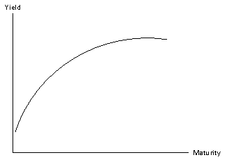
Historically, the U.S. yield curve has been upward-sloping. This is the how the yield curve normally looks, it has been referred to as the ‘normal yield curve’. The yields of longer-maturity bonds tend to be higher than the yields of shorter-maturity bonds since the longer maturity bonds are riskier. This is because:
- Changes in market conditions have a greater impact on the prices of longer maturity bonds than shorter maturity bonds; and
- There is more uncertainty over market conditions that take place further in the future.
The shape and level of the yield curve can change over time. If economic activity is expected to accelerate in the future, the yield curve tends to become steeper, since future rates are expected to be higher than they are now. If the economy is expected to slow in the future, the yield curve tends to become flatter, since future rates are expected to be lower than they are now.
During periods of rising inflation, the entire yield curve shifts up as lenders require higher rates of return to compensate for the loss of purchasing power. During periods of falling inflation, the entire yield curve shifts down.
Occasionally, the yield curve can have a negative slope (referred to as an ‘inverted yield curve’); this tends to happen when inflation is at unusually high levels and is expected to fall in the future or when recessions are imminent (related articles on negative spreads or inverted yield curves).
2) Definitions of Interest Rates
Interest rates can be expressed in several different equivalent ways, such as:
- Discount factors
- Spot rates
- Forward rates
- Yields
The prices of Treasury securities may be used to compute discount factors, spot rates, forward rates and yields. Discount factors can be computed directly from the prices of Treasuries. Spot rates can be computed from discount factors; forward rates can be computed from spot rates.
a) Discount Factors
A discount factor represents the present value of a sum. For example, if the one-year discount factor is 0.942900, this indicates that the present value of $1 received in one year is $0.942900. Discount factors cannot exceed 1 and will fall continuously as their maturity increases.
Discount factors may be computed from the prices and coupons of Treasury securities. As an example, the following table shows the prices and coupon rates of off-the-run Treasury securities with maturities of 6 months, 12 months, 18 months and 24 months. Off-the-run securities are those that have been issued in the past; the most recently issued securities are said to be on-the-run. For example, if a one-year Treasury bill was issued six months ago, it is now considered to be an off-the-run six month Treasury bill. A newly-issued six-month Treasury bill is considered to be on-the-run.
| Maturity | Coupon Rate | Price |
| 6 months | 0.80% | $990.00 |
| 12 months | 1.40% | $975.00 |
| 18 months | 2.20% | $960.00 |
| 24 months | 2.80% | $935.00 |
Each bond has a face value of $1,000 and makes semi-annual coupon payments.
When the six month bond matures, it will pay one final semi-annual coupon along with the bond’s principal or face value of $1,000. The annual coupon rate is 0.8%, so the annual coupon payment is (0.008)($1,000) = $8. Each semi-annual coupon payment will therefore be $8/2 = $4. As a result, the bond will provide a cash flow of $1,004 in six months.
Since the price of a bond equals the present value of its promised future cash flows, the following relationship holds for the six-month bond:
990 = 1004d(0.5)
where:
d(t) = the discount factor with a maturity of t years
According to this equation, the price of the bond ($990) equals the present value of the remaining cash flow of $1,004. Since this cash flow occurs in six months, its present value is obtained by multiplying it by the six month discount factor:
1004d(0.5)
Solving for d(0.5) gives:
990 = 1004d(0.5)
d(0.5) = 990 / 1004 = 0.986056
For the 12 month bond, the following relationship holds:
975 = 7d(0.5) + 1007d(1)
This is because the bond’s price is $975. With a 1.4% annual coupon, the bond pays two semi-annual coupons each year of (1.4%/2)($1,000) = $7. This bond will make a coupon payment in six months, and then a final coupon payment and repayment of principal when the bond matures in twelve months.
Since d(0.5) = 0.986056,
975 = 7d(0.5) + 1007d(1)
975 = 7(0.986056) + 1007d(1)
975 = 6.9024 + 1007d(1)
968.0976 = 1007d(1)
d(1) = 968.0976/1007
= 0.961368
Using this same approach:
d(1.5) = 0.928366
d(2) = 0.882386
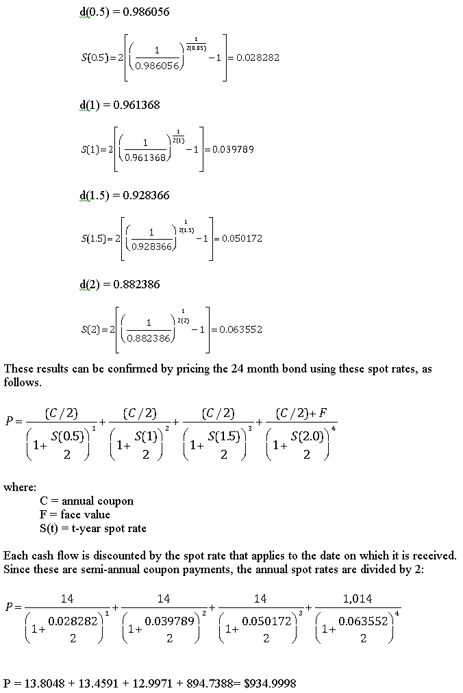
These results can be confirmed by pricing the 24 month bond using these discount factors, as follows. The 24 month bond has four remaining cash flows. The bond’s annual coupon rate is 2.8%, so that its semi-annual coupon payments equal (2.8%/2)($1,000) = $14. Therefore, the price of the bond equals:
P = 14d(0.5) + 14d(1) + 14d(1.5) + 1,014d(2)
P = 14(0.986056) + 14(0.961368) + 14(0.928366) + 1,014(0.882386)
P = 13.8048 + 13.4592 + 12.9971 + 894.7394
P = $935.00005
Except for a small rounding error, this matches the bond’s market price of $935.00.
b) Spot Rates
A spot rate of interest is the yield to maturity of a zero-coupon bond. Spot rates may be derived directly from discount factors using the following formula:
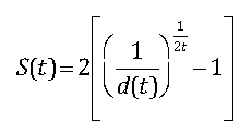
where:
S(t) = t-year spot rate
d(t) = t-year discount factor
t = maturity of spot rate (measured in years)
Based on the previous example, spot rates can be derived from the discount factors as follows:
Except for small rounding errors, this matches the bond’s market price of $935.00.
c) Forward Rates
A forward rate of interest is a rate that applies to a future time interval. For example, the rate of interest that applies to a five-year loan beginning in one year is known as a five-year rate one year forward. Forward rates are uniquely determined by the pattern of spot rates observed in the market.
As an example, suppose that a bank currently pays a 5% rate of interest for one-year time deposits, and 6% for two-year time deposits. An investor deposits $1,000 in a two-year time deposit; in two years, he will have a balance of
1,000(1.06)2 = $1,123.60.
Suppose instead that the investor deposits $1,000 in a one-year time deposit; at the end of that time, the funds are reinvested in another one-year time deposit. At the end of two years, the investor will have:
1,000(1.05)(1 + X)
The amount that the investor will have in two years cannot be determined since the one-year rate that will apply in one year is unknown. The rate of interest that equalizes the return under both scenarios is known as the one-year rate one year forward. In other words, this is the one year rate that applies one year in the future.
The one year rate one year forward can be determined by equalizing the returns to investing at the two year spot rate for two years and investing at the one year spot rate for one year and then reinvesting the proceeds for another year at the one year rate one year forward:
1,000(1.06)2 = 1,000(1.05)(1+X)
(1.06)2/(1.05) = 1 + X
0.0701 = X
The forward rate of interest can be written as f(t,T), where t is the time at which the rate begins and T is the time at which the rate matures. In this example, the one-year rate one-year forward is written as f(1,2). The one-year rate two years forward is written as f(2,3); the two-year rate one-year forward is written as f(1,3).
Forward rates can be computed directly from spot rates. Based on the previous example, the forward rates can be computed directly from the spot rates:
S(0.5) = 0.028282
S(1) = 0.039789
S(1.5) = 0.050172
S(2) = 0.063552
For example, the six month forward rate six months forward, designated f(0.5, 1) is the rate at which the following investments would provide the same rate of return:
- Investing for twelve months at the twelve month spot rate (S(1))
- Investing for six months at the six-month spot rate (S(0.5)) and then reinvesting the proceeds at the six-month forward rate six months forward (f(0.5, 1))
This implies that:
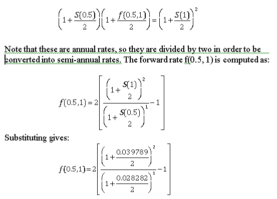
f(0.5,1) = 2[(1.040185/1.014100) – 1]
f(0.5, 1) = 0.051444
Using this same technique, the six-month forward rate one year forward is computed as:
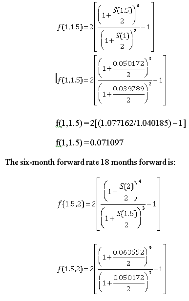
f(1.5,2) = 2[(1.133292/1.077162) – 1]
f(1.5,2) = 0.104218
These results can be confirmed by pricing the 24 month bond using these spot rates, as follows. When pricing bonds with forward rates, each cash flow is discounted by a sequence consisting of the short-term spot rate followed by the appropriate forward rates.
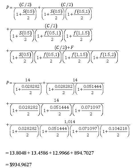
Except for rounding errors, this matches the bond’s market price of $935.00.
d) Yields
The yield to maturity (YTM) is the rate of interest at which the market price of a bond equals the present value of its expected future cash flows. Yields cannot be determined algebraically; they must be computed with a specialized financial calculator or Microsoft Excel.
As an example, the yields for the four bonds in the previous example can be computed with Excel’s YIELD function, as follows:
= YIELD(settlement, maturity, rate, pr, redemption, frequency, [basis])
where:
settlement = date on which the bond is purchased (for example, “1/1/15” represents January 1, 2015)
maturity = date on which the bond matures
rate = annual coupon rate
pr = price (as a percentage of face value); for example, if a bond has a face value of $1,000 and the price is $950, pr would be set equal to 95 (i.e., 95% of face value)
redemption = par or face value (based on 100)
frequency = coupon frequency
basis = day count convention
basis = the day-count convention; the options are:
0 = 30/360 (this is the default or assumed value)
1 = actual/actual
2 = actual/360
3 = actual/365
4 = European 30/360
For the six month, 0.80% coupon bond, the yield is computed as:
= YIELD(settlement, maturity, rate, pr, redemption, frequency, [basis])
= YIELD(“1/1/16”, “7/1/16”, 0.8%, 99, 100, 2, 0)
= 0.028283
= 2.8283%
Note that the settlement and maturity dates must be entered with quotes. Excel assigns a numerical value to each date based on a starting value of 1 = January 1, 1900. This value is increased by one for each day; for example, 2 = January 2, 1900. The numerical value of 1/1/16 is 42370 and the numerical value of 7/1/16 is 42552. These numerical values may be used for settlement and maturity.
For the twelve month, 1.40% coupon bond, the yield is computed as:
= YIELD(settlement, maturity, rate, pr, redemption, frequency, [basis])
= YIELD(“1/1/16”, “1/1/17”, 1.4%, 97.5, 100, 2, 0)
= 0.039748
= 3.9748%
For the eighteen month, 2.20% coupon bond, the yield is computed as:
= YIELD(settlement, maturity, rate, pr, redemption, frequency, [basis])
= YIELD(“1/1/16”, “7/1/17”, 2.2%, 96, 100, 2, 0)
= 0.050011
= 5.0011%
For the twenty-four month, 2.80% coupon bond, the yield is computed as:
= YIELD(settlement, maturity, rate, pr, redemption, frequency, [basis])
= YIELD(“1/1/16”, “1/1/18”, 2.8%, 93.5, 100, 2, 0)
= 0.063103
= 6.3103%
These results can be confirmed by pricing the 24 month bond using these yields, as follows. Each cash flow is discounted by the two-year yield since this is the maturity of the bond.
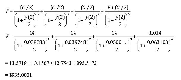
Except for rounding errors, this matches the bond’s market price of $935.00.
Unlike pricing a bond with discount factors, spot rates and forward rates, when pricing a bond with yields, each cash flow is discounted with the same yield.
Also note that the price of the 24 month bond is the same whether it is priced using discount factors, spot rates, forward rates or yields.
e) The Relationship Between Yields, Spot Rates and Forward Rates
The following chart summarizes the discount factors, yields, spot rates and forward rates for the previous set of examples. The spot rates shown are S(0.5), S(1), S(1.5) and S(2). The forward rates are f(0, 0.5), f(0.5, 1), f(1, 1.5) and f(1.5, 2). Note that f(0, 0.5) is the same as the six month spot rate, S(0.5), since it starts immediately and matures in six months. The yields are y(0.5), y(1), y(1.5) and y(2). (S(0.5) in the chart is slightly different from f(0, 0.5) and y(0.5) due to rounding errors.)
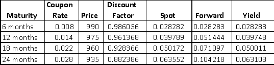
In this case, the yields are increasing with maturity; i.e., the yield curve is upward sloping. When this happens:
- The shortest maturity yield matches the shortest maturity spot rate and forward rate;
- As maturities increase, the spot curve rises above the yield curve, while the forward curve rises above the spot curve
If the yield curve is downward sloping, the reverse is true:
- The shortest maturity yield matches the shortest maturity spot rate and forward rate
- As maturities increase, the spot curve falls below the yield curve, while the forward curve falls below the spot curve
If the yield curve is flat (i.e., the yield is the same for all maturities), then:
- The shortest maturity yield matches the shortest maturity spot rate and forward rate
- As maturities increase, the yield curve, spot curve and forward curve coincide with each other and are flat
3) Theories of the Term Structure of Interest Rates
Several theories have been proposed to explain the relationship between the maturities of bonds and the rates paid by these bonds. These include:
- Expectations theory
- Liquidity premium theory
- Market segmentation theory
a) Expectations Theory
According to the Expectations Theory, long-term rates are an average of investors’ expected future short term rates of interest.
According to this theory, if the yield curve is upward sloping, this indicates that investors expect short-term rates to be higher in the future. If the yield curve is downward sloping, this indicates that investors expect short-term rates to be lower in the future. If the yield curve is flat, this indicates that investors expect short-term rates to be unchanged in the future.
One of the key assumptions of the Expectations Theory is that investors do not have any preferences for bond maturities; they are indifferent between bonds of all maturities. For example, an investor who needs to save for five years would be indifferent between:
- Buying a five-year bond
- Buying a ten-year bond and selling it after five years
- Buying a thirty-year bond and selling it after five years
The following numerical example illustrates this idea. Suppose that the current one-year rate is 9% and the current two-year rate is 10%. According to the Expectations Theory, the fact that the two-year rate is higher than the one-year rate implies that investors expect the one-year rate to be higher next year.
This can be shown by computing the return to the following strategies:
- Buying a two year bond
- Buying a one-year bond and then reinvesting the proceeds in another one-year bond
If the investor buys the two-year bond, his return over the next two years will be:
(1 + 0.10)2 – 1 = 0.21 = 21%
In order for the investor to be indifferent between the two strategies, he must expect to earn the same return from both. In order for him to earn 21% by buying a one-year bond with a 9% rate and then reinvesting in another one-year bond, the expected rate paid by the second one-year bond must be:
(1 + 0.09)(1 + X) = (1.10)2
(1 + X) = (1.10)2 / (1.09)
X = (1.10)2 / (1.09) – 1
X = 0.11 = 11%
This shows that if one year rates are 9% and two-year rates are 10%, then according to the Expectations Theory, investors expect the one-year rate to be 11% next year. When long-term rates exceed short-term rates, this indicates that investors expect future short-term rates to be greater than they are today. Equivalently, if long-term rates are below short-term rates, according to the Expectations Theory, investors expect short-term rates to be lower in the future than they are today.
b) Liquidity Premium Theory
According to the Liquidity Premium Theory, a long-term rate of interest is an average of short-term rates plus a liquidity premium. In other words, investors expect to be compensated for holding long-term bonds instead of short-term bonds as long-term bonds are perceived to be riskier. This causes the yield curve to be steeper than it would be under the Expectations Theory.
As an example, suppose that the one-year rates over the next five years are expected to be 5%, 6%, 7%, 8% and 9%, respectively. The liquidity premium for holding bonds of these maturities equals 0% for a one-year bond, 0.25% for a two-year bond, 0.5% for a three-year bond, 0.75% for a four-year bond and 1.00% for a five-year bond. What are the implied two-year and five-year rates under the:
- Expectations Theory
- Liquidity Premium Theory
Under the Expectations Theory, the implied two-year rate is computed as:
(1 + X)2 = (1 + 0.05)(1 + 0.06)
(1 + X)2 = 1.113
1 + X = 1.1131/2
X = 1.1131/2 – 1
X = 0.055 = 5.5%
Under the Liquidity Premium Theory, the implied two-year rate is computed as:
(1 + X)2 = (1 + 0.05 + 0)(1 + 0.06 + 0.0025)
(1 + X)2 = (1.05)(1.0625)
(1 + X)2 = (1.115625)
1 + X = 1.1156251/2
X = 1.1156251/2 – 1
X = 0.05623 = 5.623%
Under the Expectations Theory, the implied five-year rate is computed as:
(1 + X)5 = (1 + 0.05)(1+ 0.06)(1 + 0.07)(1 + 0.08)(1 + 0.09)
(1 + X)5 = 1.401939252
1 + X = 1.4019392521/5
X = 1.4019392521/5 – 1
X = 0.0699 = 6.99%
Under the Liquidity Premium Theory, the implied five-year rate is computed as:
(1 + X)5 = (1 + 0.05)(1+ 0.0625)(1 + 0.0750)(1 + 0.0875)(1 + 0.10)
(1 + X)5 = 1.43465889
1 + X = 1.434658891/5
X = 1.434658891/5 – 1
X = 0.0749 = 7.49%
c) Market Segmentation Theory
Under the Market Segmentation Theory, rates are determined by supply and demand conditions in each maturity range of the yield curve. For example, 30-year rates are influenced by the supply and demand for mortgages.
According to this theory, investors have a strong preference for a specific maturity and would require a premium to invest in other bonds with different maturities. As a result, there can be a risk premium for different maturities along the yield curve, but they do not necessarily increase with maturity as they do under the Liquidity Premium Theory. As a result, the yield curve may not rise or fall continuously.
This article is one part of a series on fixed income portfolios. Other articles in this series include:
- Time Value of Money – A Quick Overview;
- An Introduction to Bonds, Bond Valuation & Bond Pricing; and
- Managing Bond Portfolios: Strategies, Duration, Modified Duration, Convexity.
We have provided you with a good overview of the term structure, interest rates and yield curves. If you have questions or need help understanding the concept of term structure, how interest rates can be used or yield curves, please feel free to call or email our corporate finance tutoring team and one of our CFA or MBA tutors will be happy to assist you with private tutoring.