CFA students and MBA students that specialize in corporate finance will learn about managing fixed income or bond portfolios. This article is one part of a series on fixed income portfolios. Other articles in this series are 1) Time Value of Money – A Quick Overview, 2) An Introduction to Bonds, Bond Valuation & Bond Pricing and 3) Term Structures, Interest Rates and Yield Curves.
1) Measures of Interest Rate Risk Vs, Bond Portfolio Management Strategies
The management of bond portfolios or fixed income portfolios introduces several unique challenges; among the most important is the ability to determine the risk associated with fixed income instruments. Three of the most important measures of interest rate risk are known as:
- Macaulay duration
- Modified duration
- Convexity
These measures are widely used to determine how sensitive a bond’s price is to changes in market yields or in other words: what is the risk associated with this bond portfolio when market rates change? These measures also called interest rate risk measures quantify the bond portfolio risk. These interest rate risk measures have one major drawback: they are based on the assumption that all promised cash flows will actually materialize. This assumption is especially problematic when bonds contain embedded options, which can be used to alter the pattern of cash flows from a bond. In order to properly account for embedded options, more advanced risk measures have been developed; these are known as:
- Effective duration
- Effective convexity
The above interest rate risk measures only help you quantify understand the level of risk in a bond portfolio. They do not help you mitigate or manage the bond portfolio risk! Different types of strategies can be used to manage the returns and risk of a bond portfolio. Two of the more widely-used bond portfolio risk management strategies are:
- Indexing
- Immunization
We provide an overview of the above measures of interest rate risk and bond portfolio management strategies below.
2) Macaulay Duration
Duration is a measure of the sensitivity of a bond’s price to changes in the yield to maturity. Duration enables an investor to directly compare the risks of bonds with different face values, maturities, coupons, etc. The concept of duration was first defined by Frederic Macaulay in 1938 in his book “The Movement of Interest Rates, Bond Yields and Stock Prices in the United States Since 1856.” As a result, the form of duration that he suggested is known as Macaulay duration. Since the development of Macaulay duration, a closely related measure known as modified duration has become widely used in many applications.
Macaulay duration is the sum of the present values of a bond’s time-weighted cash flows divided by the bond’s price. In the special case of a zero coupon bond, Macaulay duration equals the bond’s maturity.
As an example, suppose that a ten-year U.S. Treasury note that was issued seven years ago with a coupon rate of 6% and a face value of $1,000. Also assume that newly-issued (“on-the-run”) three-year Treasury notes offer a coupon rate of 3%, and that the note pays semi-annual coupons.
The formula for computing Macaulay Duration is:
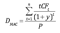
where:
DMAC = Macaulay Duration
t = a time index
n = the number of periods until the bond’s maturity date
CFt = the bond’s cash flow at time t
y = the bond’s yield to maturity
P = the bond’s price
The price of the bond is computed as the present value of the bond’s future cash flows. The bond in this example makes a semi-annual coupon payment of $30 twice per year; at maturity, the face value (principal) of $1,000 is repaid. Each cash flow is discounted by the semi-annual yield to maturity, which is one-half of 3%, or 1.5%. The results are shown in the following equation:
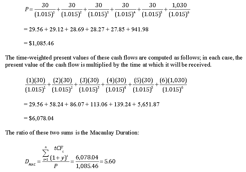
Since the bond makes semi-annual coupon payments, this result is measured in terms of semi-annual periods. The Macaulay Duration expressed in years is 5.60/2 = 2.80. This indicates that it takes 2.8 years before the present value of the cash flows adds up to 1,000, the initial price of the bond.
3) Modified Duration
Although Macaulay Duration is a useful measure of interest rate risk, for many applications the interpretation is not convenient. An alternative form of duration was developed that can be interpreted as the sensitivity of a bond’s price to a change in the yield curve. This version of duration is known as modified duration. Modified duration is computed as follows:
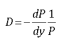
where:
D = modified duration
P = the bond’s price
dP = an instantaneous change in the bond’s price
dy = an instantaneous change in the bond’s yield
This can be approximated as:
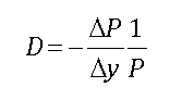
where:
DP = a small change in the bond’s price
Dy = a small change in the bond’s yield
The ratio dP/dY is known as the first derivative of the price with respect to the yield. This can be thought of as the slope of the price-yield curve, which shows the relationship between the price of a bond and the yield. An example of this is shown below:
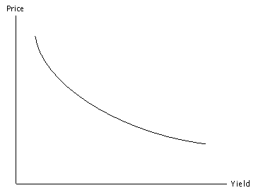
The price-yield curve is negatively sloped; in other words, the first derivative is negative throughout. The price-yield curve is also convex to the origin; this means that the curve is “bowed”, and the second derivative is positive throughout.
Modified duration equals the negative of the slope of the price-yield curve, divided by the bond’s price. The negative sign ensures that modified duration will be a positive number, which is easier to interpret than a negative number. The slope is scaled by the price to correct for the fact that not all bonds are issued with the same face value and can therefore have very different prices. The goal of modified duration is to measure the sensitivity of the bond’s price to changes in the yield curve.
Modified duration can be computed by using calculus; this is accomplished by differentiating the bond’s pricing function (the present value of the future cash flows) with respect to the bond’s yield, and then multiplying the result by –(1/P).
As a simpler alternative, the modified duration can be computed directly from the bond’s Macaulay duration with the following equation:
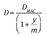
where: m = the coupon frequency
In this formula, m = 1 for a bond that pays annual coupons, and m = 2 for a bond that pays semi-annual coupons.
Based on the previous example, the modified duration is computed as follows:
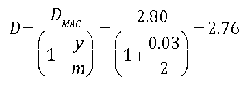
This can be interpreted as follows. If the bond’s yield rises by 1%, the bond’s price will fall by approximately 2.76%, and vice versa. Note that the smaller the change in yield, the more accurate this estimate will be.
a) Factors That Affect Modified Duration
Modified duration is a function of a bond’s maturity and coupon rate.
- Duration is an increasing function of maturity, since a longer maturity bond has more cash flows that are affected by a given change in yield.
- Duration is a decreasing function of the coupon rate. Zero coupon bonds are most heavily affected by changes in yield since all cash flows take place on a single date; with coupon-bearing bonds, the impact of changes in yield is spread out among the coupon payments.
As an example, the following table shows the modified duration of four bonds: a 5 year zero coupon bond, a 5 year 5% coupon bond, a 10 year zero coupon bond and a 10 year 5% coupon bond. The yield curve is flat at 4% (i.e., yield is 4% for all maturities.) Coupons are assumed to be paid semi-annually.
| BOND | MODIFIED DURATION |
| 5 year 0% coupon | 4.90 |
| 5 year 5% coupon | 4.41 |
| 10 year 0% coupon | 9.80 |
| 10 year 5% coupon | 7.92 |
The chart shows that the 5 year zero coupon bond has a modified duration of 4.90, which is well below the 9.80 modified duration of the 10 year zero coupon bond. Similarly, the 5 year 5% coupon bond has a modified duration of 4.41, while the 10 year 5% coupon bond has a modified duration of 7.92.
In both cases, the 10 year bond has more cash flows than the five year bond, and some of these cash flows will take place further in the future. Therefore, a given change in yield will have a greater impact on the present value of the 10 year bond’s cash flows; as a result, its price will be more sensitive to changes in yields than the 5 year bond.
The chart also shows that the 5 year zero coupon bond has a modified duration of 4.90, which is greater than the 4.41 modified duration of the 5 year 5% coupon bond. Similarly, the 10 year zero coupon bond has a modified duration of 9.80 compared with a modified duration of 7.92 for the 10 year 5% coupon bond.
In both cases, the zero coupon bond has a higher duration than the 5% coupon bond. This is because with a zero coupon bond, all cash flows take place at maturity; as a result, a given change in yield has a greater impact on the present value of the cash flows than it does for a bond with a higher coupon and the same maturity.
b) Using Modified Duration to Estimate Changes in Bond Prices
Based on the formula for computing modified duration, the approximate change in the price of a bond may be estimated from the bond’s modified duration, price and the change in yield. Since
The change in a bond’s price due to a given change in yield can be determined by rearranging this equation algebraically:
As an example, suppose that for the ten-year U.S. Treasury note that was issued seven years ago with a coupon rate of 6% and a face value of $1,000, the yield rises from 3% to 3.01%. What will be the impact on the price of the bond? The change in yield is computed as:
Δy = 0.0301 – 0.0300 = 0.0001
This is 0.01%, which is also known as a basis point. One hundred basis points equal one percent. Therefore, the change in the bond price will be:
ΔP = -(2.76)(1,085.46)(0.0001)
= -$0.30
The price will fall by about thirty cents as a result of an increase of one basis point in the bond’s yield. The new price will be approximately $1,085.46 – $0.30 = $1,085.16.
In order to determine the percentage change in a bond’s price due to a given change in yield, the following equation can be used:
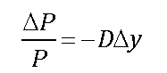
The change in P divided by the original price of P gives the percentage change in the price. Based on the previous example:
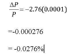
The price of the bond falls by about 0.0276% as a result of an increase in the yield by one basis point.
4) Convexity
A bond’s convexity refers to the sensitivity of the bond’s modified duration to changes in yield. Based on the price-yield curve:
- at low yields, the modified duration changes very quickly as the yield changes (since the price-yield curve is very steep); therefore, the convexity is high
- at higher yields, the modified duration changes very slowly as the yield changes (since the price-yield curve is relatively flat); therefore, the convexity is low
The formula for computing convexity is:
As an example, suppose that the price of a bond is initially P0, and then changes to P1. In this case, the first difference of P equals DP = P1 – P0. Suppose the bond price now changes from P1 to P2. There have now been two changes: DP1 = P1 – P0 and DP2 = P2 – P1. The second difference of P equals:
Δ2P = ΔP2 – ΔP1
= (P2 – P1) – (P1 – P0)
= P2 – 2P1 + P0
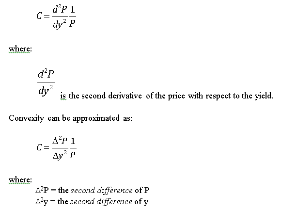
Convexity can be computed by using calculus; this is accomplished by computing the second derivative of the bond’s price function with respect to the bond’s yield, and then multiplying the result by 1/P. As a simpler alternative, the convexity can be computed with the following equation:
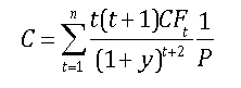
where:
C = convexity
t = a time index
n = the number of periods until the bond’s maturity date
CFt = the bond’s cash flow at time t
y = the bond’s yield to maturity
P = the bond’s price
Using the example of the ten-year U.S. Treasury note that was issued seven years ago with a coupon rate of 6%, a face value of $1,000 and a yield of 3%, the convexity can be computed as follows.
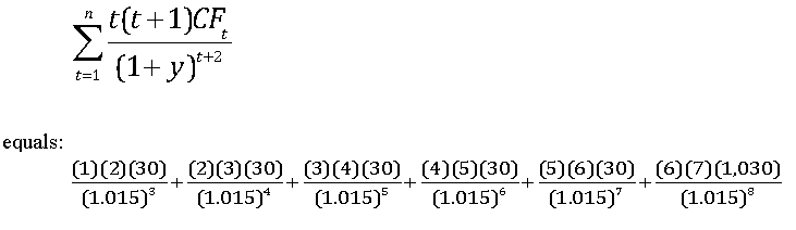
= 57.38 + 169.59 + 334.17 + 548.73 + 810.92 + 38,402.38
= $40,323.18
When this is multiplied by 1/P, the convexity is determined to be:
C = 40,323.18 / 1,085.45 = 37.15
Convexity is positive for option-free bonds. Convexity can be negative if a bond contains an embedded call option. An embedded call option enables the issuer to repurchase the bond at a fixed price (known as the call price) at a specified time in the future. With very low yields, the likelihood of a bond being called is extremely high; as a result, investors will not pay more than the call price for a bond, no matter how low yields are. This results in a phenomenon known as “price compression”, in which the price of a bond is prevented from rising above the call price while the price can still fall due to rising yields. When yields are extremely low, the bond’s convexity can become negative as the price curve flattens out.
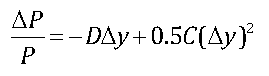
Using both modified duration and convexity to estimate the change in a bond’s price due to a given change in yield can be estimated more precisely than with modified duration alone; the equation is:
For the ten-year U.S. Treasury note that was issued seven years ago with a coupon rate of 6%, a face value of $1,000 and a yield of 3%, the change in the price due to an increase in the yield to 3.01% can be computed as follows:
ΔP = -2.76(1,085.46)(0.0001) + 0.5(37.15)(1,085.46)(0.0001)2
= -0.30 + 0.0002
= -$0.2998
In this case, using convexity in addition to modified duration added very little accuracy to the estimated price change. In other cases, using convexity can make a significant improvement in the estimation of the price change. This can occur when the convexity is very large; unlike modified duration, which cannot exceed the maturity of the bond, the convexity of a bond can reach a value in the thousands.
In addition to computing the change in a bond’s price due to a given change in yield, modified duration and convexity can be combined to give the approximate percentage change in the price of a bond, as follows:
5) Effective Duration and Convexity
One of the major drawbacks of the modified duration and convexity measures is that they are based on the assumption that all promised cash flows to a bond will actually be made. This is not necessarily the case for a bond containing an embedded option. In particular, with an embedded call option, the bond can be repurchased prior to maturity by the issuer. This will result in the last few years’ worth of cash flows not being received by the bond owner. As a result, the modified duration and convexity measures may not accurately reflect the risk of this bond.
In order to correct for this problem, two alternative measures were developed: effective duration and effective convexity. With these measures, a model of the term structure of interest rates is needed. Within the model, yields are increased by a specified number of basis points, and the impact on the price is observed. Yields are then decreased by the same number of basis points, and the impact on the price is observed. Effective duration is defined as follows:
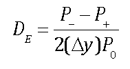
where:
DE = effective duration
P0 = the initial price of a bond
P– = the price of the bond after the yield curve shifts down by Δy basis points
P+ = the price of the bond after the yield curve shifts up by Δy basis points
Dy = the change in yield
For example, suppose that a bond’s price is currently $1,050.00. If the yields in a term structure model are reduced by 25 basis points, the bond’s price rises by $26.25 to $1,076.25. If the yields are increased by 25 basis points, the bond’s price falls by $25.89 to $1,024.11. In this case, the effective duration would be:
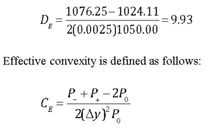
where:
CE = effective duration
6) Passive Bond Portfolio Strategies
Different types of strategies can be used to manage the returns and risk of a bond portfolio; some of the more widely-used strategies are known as:
- Indexing
- Immunization
With an indexing strategy, the portfolio manager attempts to replicate a bond index, such as the Standard and Poor’s 500 Bond Index. Due to the varied features of bonds, this is a more difficult objective to accomplish than replicating a stock market index. With an immunization strategy, the risk of a portfolio is managed by attempting to ensure that the duration of a bond portfolio matches a specified investment time horizon. The goal is to ensure that the portfolio will provide a certain rate of return by the end of the time horizon.
This article is part of a series on fixed income portfolios. Other articles in this series include:
- Time Value of Money – A Quick Overview;
- An Introduction to Bonds, Bond Valuation & Bond Pricing; and
- Term Structures, Interest Rates and Yield Curves.
We have provided you with a quick introduction the measures of interest rate risk and bond portfolio management strategies used to manage fixed income risk. If you have questions or need help understanding these topics, please feel free to call or email our corporate finance tutoring team and one of our CFA or MBA tutors will be happy to assist you with private tutoring.