The Time Value of Money (“TVM”) is a concept on which the rest of finance theory rests on. Therefore, it is critical that students understand this concept well. We expand on the Time Value of Money under the following headings:
- What does the “Time Value of Money” mean or capture?
- Why does the Value of Money Decline?
- The Present Value Formula
- Infographic on the Time Value of Money
- Computing the Time Value of Money
- Interest Rates and Compounding Frequencies
- Interest Rate Conventions
- Continuous Compounding
1) What does the “Time Value of Money” mean or capture?
Most students agree that what $10 will buy you today will be more than what $10 will buy in 5 years in the future. Similarly, they also agree that $10 would have gotten them a lot more 5 years ago than it will today. Since they agree that this is true, I tell them that they have understood the time value of money concept! This is exactly what the concept of the time value of money in finance captures: As time flows, the value of money declines. (Article Index)
2) Why does the Value of Money Decline?
The value of money declines due to the combined impact of the following:
- Inflation in the economy;
- Risks involved in delayed receipts of cash or financial transactions; and
- Opportunity cost of capital.
While each of these forces alone can cause the value of money to decline individually, all three factors, inflation, risk, and opportunity cost of capital, act with different strength to cause a decline in the value of money as time flows. (Article Index)
3) The Present Value Formula
The present value formula quantifies how fast the value of money declines. This formula shows you how much one single cash payment received in the future (FV) at the time period (t) is worth in today’s terms (PV).
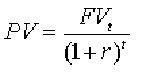
Present Value (PV) stands for the value of the money in today’s terms.
Future Value (FV) stands for the amount of cash received in the future.
The discount rate (r) is the rate at which the value of money is declining.
The time period (t) is the unit of time when the future value or cash is received.
Computing the present value of a sum of money received in the future (future value) is known as discounting. We say we are discounting the future value to its equivalent value today to account for inflation, risk, and opportunity cost. In other words, we will be indifferent to receiving the present value now or the future value at a future point in time. (Article Index)
4) Infographic on the Time Value of Money
The GraduateTutor.com finance team has put together this infographic on the Time Value of Money for the visual learners. We have a follow up infographic on the commonly used Time Value of Money formulas.
Please feel free to embed this infographic using the code below this post. Do provide us credit for this poster by linking to us.
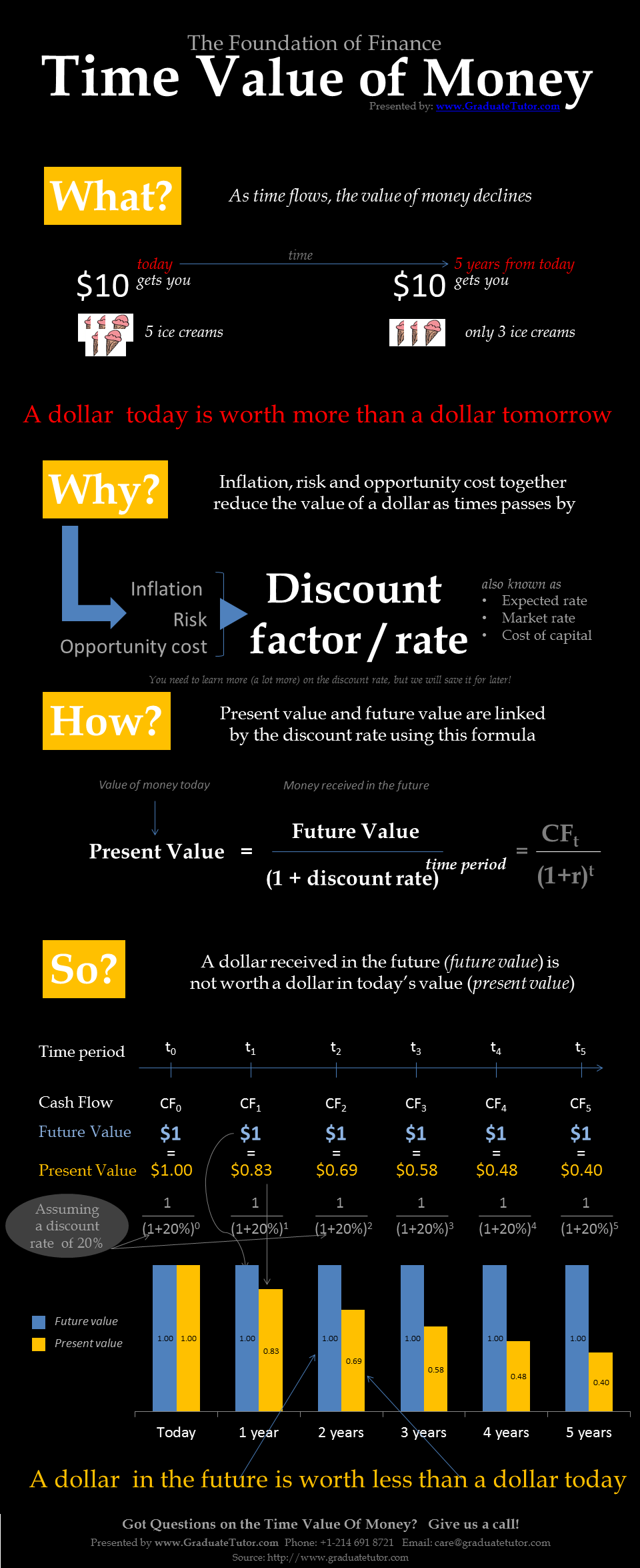
Time Value of Money – An infographic by the finance tutoring team at GraduateTutor.com. (Article Index)
(Content below is contributed by Prof. Alan Anderson)
5) Computing the Time Value of Money: Discounting vs. Compounding
If a sum of money is invested today, it will earn interest or a return on the investment, increasing in value over time. The value that the sum grows into is known as its future value. Computing the future value of a sum of money invested today (present value) is known as compounding.
The present value of a sum of money received in the future (future value) is the amount that would need to be invested today in order to be worth that sum in the future. Computing the present value of a sum of money received in the future (future value) is known as discounting. We say we are discounting the future value to its equivalent value today to account for inflation, risk, and opportunity cost. In other words we will be indifferent to receiving the present value now or the future value at a future point in time.
The Future Value of a Sum of Money Invested Today
The future value of a sum of money invested today (present value) depends on 1) the interest rate earned and 2) the interval of time over which the sum is invested. The relationship between the future value and present value is captured in the following formula:
FVt = PV*(1+r)t
where:
- FVt = future value of a sum invested for t periods
- r = periodic interest rate
- PV = present value
- t = number of periods until the sum is received
The time period may be a year, a month, a week, etc. The rate and time period used in the future value formula must be consistent: for example, if time (t) is measured in months, then the rate (r) must be a monthly rate.
As an example, suppose that a sum of $1,000 is invested for four years at an annual rate of interest of 3%. What is the future value of this sum? In this case, t = 4, r = 3% and PV = $1,000.
FVt = PV(1+r)t
FV4 = 1,000(1+.03)4
FV4 = 1,000(1.12551)
FV4 = $1,125.51
The Present Value of a Sum
The value of a sum of money today, referred to as present value, that is expected to be received at a point in time in the future (future value), depends on 1) the interest rate earned and 2) the interval of time over which the sum is invested. The formula for computing the present value of a sum of money received in the future is:
Note that the present value is simply the inverse of the future value. We arrive at the present value and future value formulas by rearranging the same equation.
As an example, how much must be deposited in a bank account that pays 5% interest per year in order to be worth $1,000 in three years? In this case, t = 3, r = 5% and FV3 = $1,000.
Present Value of (or what must be deposited to get) $1,000 in three years= 1,000/(1.1576) = $863.84 (Article Index)
6) Interest Rates and Compounding Frequencies
Compounding refers to the frequency with which interest rates are charged or paid during a given year. In practice, interest rates can be compounded anywhere from once per year to once per day; the theoretical limiting case is known as continuous compounding, in which rates are compounded at every instant in time. Compounding frequency is one of the most important determinants of the future value and the present value of a sum.
For example, if a bank offers a 4% rate of interest with annual compounding, an investor who holds $1,000 in the bank for one year will have a balance of: $1,000(1 + 0.04) = $1,040 at the end of the year. In other words, the future value of this sum is $1,040.
If the interest is compounded semi-annually, then the investor will receive half of the annual rate twice per year; i.e., 2% every six months during the year. At the end of six months, the investor will have a balance of: $1,000(1 + 0.02) = $1,020 at the end of the year, the investor will have a balance of: $1,020(1 + 0.02) = $1,000(1 + 0.02)(1 + 0.02) = $1,000(1 + 0.02)2 = $1,040.40
In this case, since the principal is $1,000, the total interest is $40.40. Of this:
$40 is simple interest (interest on principal)
$0.40 is compound interest (interest on interest)
In this case, the investor received an interest payment of $1,000(0.02) = $20 at the end of six months, for a balance of $1,020. The interest payment at the end of the year was based on the principal ($1,000) and the interest ($20) in the account. The interest paid on the principal was $1,000(0.02) = $20 and the interest paid on the interest was $20(0.02) = $0.40. Combined with the $20 interest paid at the end of six months, the total interest paid during the year was $20 + $20 + $0.40 = $40.40. Of this, the $40 was based on the principal; this is the simple interest. The remaining $0.40 was based on the interest earned during the year; this is the compound interest.
As the compounding frequency increases, the simple interest earned during a given period remains fixed, but the compound interest increases. For example, with quarterly compounding, the investor in the previous example will receive 1% every three months; at the end of the year the investor will have a balance of:
$1,000(1 + 0.01)(1 + 0.01) (1 + 0.01)(1 + 0.01)
= $1,000(1 + 0.01)4 = $1,040.60
In this case, the total interest is $40.60. Of this:
$40 is simple interest (interest on principal)
$0.60 is compound interest (interest on interest)
This demonstrates an important result: as the compounding frequency increases, the future value of a sum increases.
As another example, suppose that a sum of $1,000 is invested for two years at an annual rate of interest of 8%. What is the future value of this sum based on the following compounding frequencies?
- Annual compounding
- Semi-annual compounding
- Monthly compounding
With annual compounding, t = 2, r = 8% and PV = $1,000.
FVt = PV*(1+r)^t
FV2 = 1,000*(1+.08)^2
FV2 = 1,000*(1.16640)
FV2 = $1,166.40
With semi-annual compounding, t = 4, r = 4% and PV = $1,000. The time frame is now 4 semi-annual periods, and the rate of interest is 4% per semi-annual period.
FVt = PV*(1+r)^t
FV4 = 1,000*(1+.04)^4
FV4 = 1,000*(1.16986)
FV4 = $1,169.86
With monthly compounding, t = 24, r = 0.6667% and PV = $1,000.
FVt = PV*(1+r)^t
FV24 = 1,000*(1+.006667)^24
FV24 = 1,000*(1.17289)
FV24 = $1,172.89
These results show that the future value of a sum continues to increase as the compounding frequency increases.
For the present value, a higher compounding frequency reduces the present value. This is because more compound interest is earned, which reduces the amount that must be saved today to be worth a specified sum in the future.
As an example, suppose that an investor has a target of $100,000 in five years, and can invest in a bank account that pays an annual rate of interest of 6%. How much must the investor save today in order to reach this goal based on the following compounding frequencies?
- Annual compounding
- Semi-annual compounding
- Monthly compounding
With annual compounding, t = 5, r = 6% and FV5 = $100,000.
PV = FVt / (1+r)^t
PV = 100,000 / (1+.06)^5
PV = 100,000 / 1.33823
PV = $74,725.82
With semi-annual compounding, t = 10, r = 3% and FV10 = $100,000.
PV = FVt / (1+r)^t
PV = 100,000 / (1+.03)^10
PV = 100,000 / 1.34392
PV = $74,409.39
With monthly compounding, t = 60, r = 0.5% and FV60 = $100,000.
PV = FVt / (1+r)^t
PV = 100,000 / (1+.005)^60
PV = 100,000 / 1.34885
PV = $74,137.22 (Article Index)
7) Interest Rate Conventions
Interest rates for loans, bank accounts, etc. can be quoted in two basic ways:
- Annual percentage rate (APR)
- Effective annual rate (EAR)
The annual percentage rate reflects the simple interest of a loan or an investment, while the effective annual rate reflects both the simple and compound interest.
Converting APR to EAR
In order to compare interest rates with different compounding frequencies, they can be converted into an effective annual rate (EAR); this reflects the true cost of borrowing (or the return to lending) when interest is compounded more than once per year. EAR is computed from APR as follows:
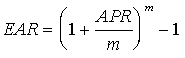
where:
m = the number of compounding periods per year
As an example, suppose that a bank charges an APR of 6% per year, compounded quarterly for a loan, what is the effective annual rate? This can be determined as follows:
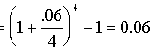
This indicates that the borrower is actually paying 6.136% per year for this loan.
Converting EAR to APR
An effective annual rate may be converted to an annual percentage rate by inverting the previous formula:
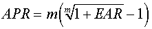
As an example, if a bank charges an EAR of 5.25% per year, compounded monthly for a loan, what is the annual percentage rate? This can be determined as follows:
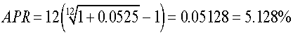
8) Continuous Compounding
Continuous compounding is the limit of compounding frequency. Continuous compounding indicates that interest rates are being compounded at every instant in time, which implies that interest is compounded an infinite number of times. A compounding frequency which is not continuous is said to be discrete. For example, annual compounding, monthly compounding, daily compounding, etc. are all examples of discrete compounding.
Using continuous compounding requires a new set of formulas for computing the future value of a sum, the present value of a sum, EAR and APR.
Computing the Future Value of a Sum with Continuous Compounding
If interest rates are compounded continuously, the future value of a sum is:
FVt = PV*(e^rt)
where:
e is a constant that is approximately equal to 2.71828
As an example, suppose that a bank offers a rate of interest of 6%, compounded continuously. An investor who deposits $1,000 in this bank for two years will have an ending balance of: FVt = 1,000(e(0.06)(2)) = $1,127.50
Computing the Present Value of a Sum with Continuous Compounding
The present value of a sum with continuous compounding is:
PV = FVt*(e^-rt)
As an example, suppose that a bank offers a rate of interest of 8%, compounded continuously. An investor who needs to have $10,000 in three years will have to save the following amount today in order to reach this goal: PV = 10,000(e^-(0.08)(3)) = $7,866.28
Computing EAR with Continuous Compounding
If interest rates are compounded continuously, EAR is computed as follows:
EAR = eAPR – 1
As an example, if a bank charges an APR of 4% per year, what is the EAR with continuous compounding?
EAR = e^APR – 1
= e^0.04 – 1
= 1.04081 – 1
= 0.04081 = 4.081%
Computing APR with Continuous Compounding
If interest rates are compounded continuously, APR is computed as follows:
APR = ln*(1 + EAR)
As an example, if a bank charges an EAR of 3.5% per year with continuous compounding, what is the APR?
APR = ln*(1 + EAR)
= ln(1.035)
= 0.03440
= 3.440% (Article Index)
Next Steps: Now that you have a good understanding of what the time value of money is and the associated concepts, why not continue to read related topics? You can either proceed to learn more about:
- Fixed Income Securities; which includes:
- How to read financial statements; which includes:
- Learning how to read a balance sheet; or
- Learning how to read a cash flow statement; or
- Learning how to understand and interpret percentage statements.
If you have more questions on the time value of money, feel free to call our accounting or finance teams and we will be happy to assist you.