All MBA students will encounter linear programing in one or more operations management courses in business school. Performing a linear programing model is one challenge. You can read our top tips to set up a linear programing model here. Interpreting the linear programing model’s solver reports present another challenge. Solver reports include a Sensitivity Report, an Answer Report and a Limits Report. This article shows you how to interpret a linear programing model’s Sensitivity Report, Answer Report and Limits Report.
We will look at the Answer Report, Sensitivity Report and Limits Report one by one starting with the Sensitivity Report.
Interpreting the Sensitivity Report
The Sensitivity Report is the most useful of the three reports. It is very useful for managerial decisions. The sensitivity report is broken down into two parts. The variable cells and constraints section.
Variable Cells Section in the Sensitivity Report
What does the Reduced Cost Tell Us?
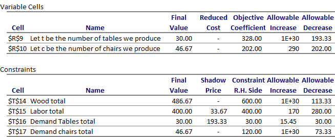
The primary values of interest in the variable cells section of the sensitivity report are the “Reduced Cost” values for each of the decision variables chosen in the linear programing model. The reduced cost value for each decision variable tells you how much your objective function value will change for a one unit increase in that decision variable.
The reduced cost for decision variable A in this example is zero. Let us see how we can interpret the reduced cost if the reduced cost for the number of tables we produce was instead a negative value: -13.58. A reduced cost of -13.58, would indicate that a one unit increase in the final value of the tables decision will result in a decrease of the objective value by 13.58. The objective value in this example is profits and so we would see a reduction in profits of 13.58 if we produce one additional table.
Objective Coefficient
The Objective Coefficient is the coefficient of the decision variables in the linear programing equation that you set up and ran on solver.
You were trying to maximize profits in this example. The profits considered the revenues and costs of machine time and material. The Objective Coefficient of 328 indicates that for each unit of decision variable A, which is the number of tables we produce in this example, your profit went up by 328.
However, this Objective Coefficient value has not considered the opportunity cost of producing one additional unit. The reduced cost discussed above has considered the opportunity cost of producing that unit too.
Allowable Increase And Allowable Decrease
The allowable increase and allowable decrease values tell you how much the objective coefficient of a decision variable can change before the recommended solution (decision variables) will change. In other words, if the objective coefficient of decision A increases by an amount less than the allowable increase, the recommended solution to the model/problem (optimal decision variables) will not change. However if the objective coefficient increases by an amount greater than 13.58, you will see that the final value for decision A will change from what is optimal now.
In this example, you will note that the allowable increase for decision variable A (tables) is a very large number and the allowable increase for decision variable B (chairs) is 290. This indicates that the recommended decision variables will not change even if A increases by a very large amount. Whereas if the objective coefficient of decision B increases by lets say 290 units or more, the recommended solution to the model/problem (optimal decision variables) will change.
However, if the objective coefficient decreases by 193.33 units for A or 202 units for B, you will see that the optimal solution recommended will change from what is recommended now.
Constraints Section in the Sensitivity Report
The second section in a Sensitivity Report is the Constraints section. The Constraints section of the Sensitivity Report provides you with the final values, the Shadow Price, the right hand side constraint and the allowable increase and decrease for each of the linear programing model’s constraints.
What does the Shadow Price Tell Us? How can we use the Shadow Price?
The primary values of interest in the Constraints section of the sensitivity report are the “Shadow Price” values for each of the constraints in the linear programing model. The shadow price for each constraint variable tells you how much your objective function value will change for a one unit increase in that constraint.
Note that we have no shadow price for wood but have a shadow price of 33.67 for labor. Notice, the constraints section, that the final value and the right hand side value of labor is 400 indicating we have used all the available labor we have. The shadow price of 33.67 for the labor in this example indicates that for every additional unit of labor we obtain will result in an increase of 33.67 in the objective value. This shadow price indicates our profits (objective function) will increase by $33.67 for every additional unit of labor added.
On the other hand, a shadow price of zero for the wood indicates that an additional unit of wood does not increase our profits or objective function. Notice, the constraints section, that the final value of wood is 486.67 whereas the right hand side constraint is 600. This indicates that we have not used all the wood we have and explains why we have a shadow price of zero! More wood will only add to our unused wood stockpile!
Constraint R.H. Side
The R.H. Side constraint is the right-hand side of that constraint equation in the linear programing model that you set up and ran on solver.
You were told in the question you had only 600 units of wood and 400 units of labor available. In addition, you were told that the maximum number of tables demanded was 30 tables and the maximum number of chairs demanded was 120 chairs. These are the values you find in the R.H. Side constraint.
Allowable Increase And Allowable Decrease
The allowable increase and allowable decrease values tell you how much the right-hand side constraint can change before the shadow price becomes unreliable (or changes). In other words, if the right-hand side constraint increases by an amount less than the allowable increase, the shadow price will not change and is relevant. However, if the right-hand side constraint increases by an amount greater than the allowable increase or decreases by an amount more than the allowable decrease, the shadow price changes and will not hold any more.
In this example, you will note that the allowable increase for labor is 170 and allowable decrease for labor is 280. This indicates that as long as the labor available increases by less than 170 or decreases by less than 280, the shadow price of 33.67 holds true. Since the shadow price holds within this range, I can estimate the increase in profits if I add 10 units of labor using the shadow price and know that the profits go up by 10*33.67= 336.7! However, if the labor availability increased by 200 units, the shadow price of 33.67 will not be valid anymore. Since the shadow price is not valid anymore, I cannot estimate the increase in profits using the shadow price of 33.67.
The Answer Report
The Answer Report is not particularly useful because most of what the Answer Report provides will already be evident to you when you look at the solver optimized model.
Your eyes will naturally drift to the objective cell to see what the maximum or minimum value your target objective cell is when your solver program has run its course. You then instinctively look for the decision variables that will get you the indicated objective value you were trying to maximize or minimize. You would have followed that up by trying to understand which of your constraints were binding or limiting you to the specified objective value. These are going to be repeated in the Answer Report!
So on first glance, Answer Report does not seem very useful. However, the Answer Report does layout the details more clearly and provide you some other details that are not evident in the Excel model.
It starts by laying out the details of the linear programing model that was run. It specifies the date and time and states the results of the run. “Solver found a solution. All Constraints and optimality conditions are satisfied.” Or otherwise…. The Answer Report indicates the model that was use: Simplex LP, GRG nonlinear or Evolutionary? The Answer Report also specifies how much time the model took, the number of iterations run and provides other options available to you.
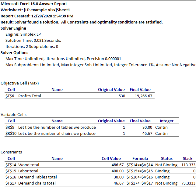
The Answer Report then goes on to detail the original value and final value of the objective function and the decision variables. It also specifies if the decision variables were specified to be integers, All different or binary.
The Answer Report then goes on to discuss the constraints. Here the Answer Report does not provide the original values but gives you the final values, the formula used and indicates if each constraint was binding or not binding. This section also tells you if the constraint had “slack” – excess or unused quantities of each constraint. In this example, you can see that the labor available and demand for tables are the binding or limiting constraints. Whereas, wood available and demand for chairs are “Not binding” and have slack or unused quantities available.
Limits Report in LP Solver Model
The third report that Microsoft Excel’s Solver add in spits out is the Limits Report. The Limits Report is not as useful as the Sensitivity Report.
The first section of the Limits Repot only provides you with the final value of the objective function. In our example the profits you will make with the optimal solution of 30 tables and 46.67 chairs will be $19,266.67.
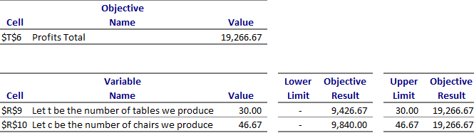
The second section of the Limits Report is the Variable Cells section. It provides you with the final values of the decision variables in the LP model. This section also tells you what the lower limit and upper limit of the decision variables would be and what the corresponding profits will be at these lower and upper limits with no other changes made. For example we can see that the objective function or profits will be 9426 if we produce no tables keeping chairs constant at 46.67.
Operations Research Tutoring
Do email or call us if we can assist you understand on interpret a linear programing models output. Our operations research tutors will be glad to walk you through a linear programing model’s sensitivity analysis, answer report and limits report using Microsoft Excel’s Solver. Other operations topics we can assist you include queuing theory and waiting lines, decision trees, linear programing using Microsoft Excel’s Solver, newsvendor models, batch processing, Littlefield simulation games. etc. Feel free to call or email if we can be of assistance with live one on one tutoring.