MBA students encounter queuing theory and waiting line formulas in a variety of operations courses with titles such as Operations Management, Supply Chain Management, Service Operations Management, Business Analytics, Decision Modelling, Management Science, Data Analytics for Operations, Technology and Operations Management, Business Process Management, Strategic Operations Management, etc.
As MBA tutors, our operations research tutors provide live online tutoring for queuing theory and waiting line one-on-one.
What is Queuing Theory & Waiting Line Studies in Operations Research
Queuing theory studies in operations research the movement of customers (people, applications, products) in a line across a system or operation to help the business manage its service quality and cost-effectively. Queuing Models help managers make decisions about capacity costs, staffing, scheduling, and other customer service aspects of operations. Queuing and waiting line models are used in a variety of industries including banks, aviation, telecommunications healthcare, and government sectors. Examples of how queuing models are used in the healthcare industry can be seen in this paper by Linda Green from Columbia University: “Queueing Theory and Modeling.”
Key Insights: Tutoring for Queuing Theory & Waiting Line Systems
As business school tutors, we emphasize the following key insights that MBA students and decision-makers must be aware of when making decisions about operations.
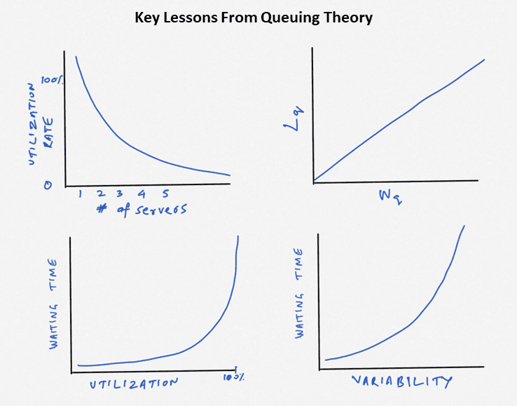
- Higher utilization increases waiting time at an increasing rate (bottom left).
- Higher variability increases waiting time at an increasing rate (bottom right).
- Higher capacity or a higher number of servers lowers the utilization rate. This also allows you to handle variability better (top left).
- Higher the waiting time, higher the number of customers waiting in line (Little’s Law)
Queuing Theory / Waiting Line Questions
As business school students, you are being trained to answer questions that impact a business operation. Some examples of questions that matter to managers and customers include:
- On average, how many customers are waiting for service?
- On average, how long are customers waiting for service?
- How many servers are needed to service customers?
- How many servers are needed if we have to reduce waiting time to a target level?
- What is the utilization level of our operations?
- What is our idle time now?
- What impact will different queuing rules have on operational performance metrics?
- Should we have separate queues or one combined queue?
- How does variability in customer arrivals affect waiting times?
- How does variability in service times affect waiting times?
- What is the cost-of-service operations?
Little’s Law vs. Queuing Theory: Different or Same?
Little’s Law is a specific formula within the broader context of queuing theory. While Little’s Law provides a useful relationship between key metrics in a queuing system, queuing theory encompasses a wider range of concepts and models for a more comprehensive analysis of queuing systems. Little’s Law is one tool within the broader framework of queuing theory.
We cover tutoring for Little’s Law and Little’s Law simulation games in more depth here.
Line Metrics/Queue performance indicator in Queuing Theory
Quantifying service quality in operations is needed to improve performance. When tutoring on queuing theory or waiting line case studies, we use the following metrics or queue performance indicators to evaluate operations.
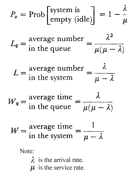
- Number of customers in service (Ls): Customers in service gives you the average number of customers currently served. This does not include the customers presently waiting in queue.
- Utilization rate (u): Utilization rate gives the percentage of time that servers are busy and not idle.
- Number of customers in the system (L): Customers in the system gives you the total number of customers in line plus the number of customers being served now on average.
- Number of customers in queue (Lq): Customers in queue gives you the average number of customers waiting in line. This does not include the customers being served currently.
- Waiting time in the queue (Wq): The Waiting time in the queue gives you the average or expected waiting time in the queue.
- Time in the system (W): The time in the system gives you the total time a customer can expect to be in the system (waiting in line and getting service).
What are the Building Blocks for Waiting Lines/Queuing Theory
There are a number of variables and patterns involved in queuing or waiting line theory. However, the three basic components of queuing or waiting line theory are:
- Arrival rate (or reciprocal of average interarrival time)
- Service rate (or reciprocal of average service time)
- Number of servers
There are many other factors to consider in practice. Some examples included in more advanced queuing and waiting line studies include:
- Underlying distributions of arrival rate
- Underlying distributions of service rate
- Coefficient of variation of arrival rate
- Coefficient of variation of service rate
- Queue discipline
Assumptions Underlying Queuing Theory/Waiting-Line Formulas
A wide variety of queuing models exist in academic literature. Each of these models are built on underlying assumptions that reflect specific operational situations or factors. Here are common assumptions that apply to queuing theory and waiting line models.
- There is a queue or line that customers join on arrival. There can be one or more queues.
- No balking: Balking is when customers arrive and leave without joining the queue.
- No reneging: Reneging is when customers in the queue leave due to frustration or impatience before being served.
- No recycling: Recycling is when customers rejoin the queue after receiving service.
- First come, first served. Customers who arrive first are served first from a queue.
- Servers perform identical services.
- Customers move to a server for service as it frees up.
- There may be one or multiple servers working in parallel.
- The arrival rate is known or specified. The reciprocal value of the arrival rate is called the inter-arrival time.
- The service rate is known or specified. The reciprocal value of the service rate is called the service time.
- Assumes a steady state, which means that the capacity of the system is higher than the arrival rate. If this is not true, you will end up with infinite lines.
Queuing Formulas
Queuing formulas estimate various queuing performance metrics, such as the average number of customers waiting in line, the average time customers spend waiting in line, etc. These formulas are a function of the utilization, the number of servers, the arrival rate, the service rate, and the variability in arrivals and service times.
Below is a sample list, but remember that there can be variations depending on the assumptions involved, including arrival and service distributions, queuing models based on the number of lines, servers, queue discipline, etc.
Source: Portland State University
Littles Law
Little’s Law, proven by John D. C. Little in 1961, shows the length of a line is directly related to the time spent in the line. Little’s Law establishes a relationship between the average number of items in a queue (L), the average rate at which items arrive (Lambda), and the average time an item spends in the system (W).
With this equation, if you know any two parameters, the third can be computed. For example, if we know that the average length of the line at ABC bank is five customers, and we know that the average time spent in line is 10 minutes, we can infer the arrival rate:
In this case, you have the average length of the line (L) as five customers and the average time spent in line (W) as 10 minutes. Plugging these values into the formula, you can solve for the arrival rate (Lamda): 5=arrival rate x 10. Solving for customers’ arrival time, we can conclude that the arrival rate at the ABC bank is 0.5 customers per minute.
The Coefficient of Variation (CV) and Waiting Lines
The coefficient of variation (CV) is a ratio that captures the variability of a data set in relation to the mean. It is calculated as the ratio of the standard deviation to the mean and is often expressed as a percentage. The formula for the coefficient of variation is the standard deviation divided by the mean.
A higher coefficient of variation indicates more significant relative variability in the data, while a lower coefficient of variation suggests less relative variability. When considering queues, utilization, length of queues, and waiting time in a system, the coefficient of variation can have several implications:
Queues and Waiting Time: A higher coefficient of variation in service times can lead to more variability in the length of queues. In systems with high variability, there may be periods of congestion and longer waiting times for customers. Conversely, a lower coefficient of variation in service times implies more predictable service and, consequently, more stable queue lengths and waiting times.
Utilization: Utilization refers to the ratio of time a resource is busy to the total time it is available. In the context of queues, utilization is often related to the efficiency of the service process. Higher variability in service times may impact utilization, as periods of high demand may lead to congestion and lower utilization during peak times. Lower variability can result in more consistent and higher utilization rates.
In summary, the coefficient of variation is an essential factor in understanding and managing the performance of systems involving queues. Higher variability generally leads to less predictable queue lengths and waiting times, while lower variability results in more stable and manageable queues. This has implications for resource utilization and the overall efficiency of the system. When designing and optimizing systems, it’s important to consider the trade-offs between variability and performance metrics to achieve desired service levels.
Queuing Theory and Waiting Line Terms
- Idle Time: The amount of time a server is inactive while waiting for customers to arrive.
- Line Length: The number of customers or items waiting in line for a service to begin.
- Little’s Law: A formula that measures the relationship between the line length, the arrival rate, and the waiting time.
- Utilization Rate: The percentage of time on average that servers are in use.
- Waiting Time: Time spent by a customer in line before service.
What Is Steady State In the Context Of Queuing Theory
In the context of queuing theory and systems analysis, the term “steady state” refers to a condition where the system has reached a stable and consistent behavior over time. In a steady state, specific key performance measures of the system, such as queue lengths, waiting times, and utilization, remain relatively constant over time.
A system can only be in a steady state when the arrival rate is less than the service rate.
Common Courses Where Queuing Theory is Covered in Graduate Programs
Queuing theory in business schools may be taught in various courses and will vary by program and semester. Here are some examples of MBA classes or areas of study that could potentially include queuing theory:
- Operations Management: Many MBA programs offer an Operations Management course, where queuing theory might be covered as part of understanding and optimizing processes.
- Supply Chain Management: Queuing theory can be relevant in understanding and managing various aspects of supply chain processes, especially when it comes to managing demand and capacity.
- Service Operations Management: Courses focusing specifically on managing service operations often cover queuing theory, as it is highly applicable to service-oriented businesses.
- Business Analytics: MBA programs that offer courses in business analytics may include queuing theory as part of the quantitative methods used to analyze and improve business processes.
- Decision Modeling: Some MBA programs have courses in decision modeling or quantitative analysis, where queuing theory might be introduced as a tool for decision-making.
- Management Science: Queuing theory is a fundamental component of management science, and MBA programs that cover this area may include it in the curriculum.
- Data Analytics for Operations: Courses that focus on using data analytics for operational decision-making may incorporate queuing theory to optimize processes.
- Technology and Operations Management: MBA classes in technology and operations management may explore queuing theory in the context of managing technology-driven processes.
- Business Process Management: Queuing theory is often relevant in the context of business process management, and some MBA programs may cover it in courses focused on this area.
- Strategic Operations Management: Courses that examine the strategic aspects of operations management may include queuing theory as a tool for achieving operational excellence.
Queueing Network Analysis
Some operations require customers to pass through more than one station. This is a queueing network. Queueing network analysis is more specialized than the queuing theory MBA students encounter in their first year of operations.
Sample Queueing Theory Questions for Practice
- As a manager of a call center, you find that your center has the following arrival and
service characteristics: Arrival rate is 72 customers per hour, the service rate is 10
customers per hour; The coefficient of variation in the arrival rate is 1.2 and the
coefficient of variation in the service rate is 0.9. What is the waiting time in minutes
expected for customers if you have 8 employees to answer calls. How many people
are waiting on line on average? - Continuing from question 1, how many servers do you need to keep waiting time less
than 2 minutes? - (continued from Q1) Business has picked up for the bank due to a new Super Bowl
advertisement campaign. The manager reports that the number of people in que has
increased to 2 people waiting on average. What is your estimate of the arrival rate?
(hint: use goal seek) - People arrive at a bank every 12 minutes on average with a standard deviation of 5
minutes. It takes about 10 minutes to serve a customer and service time has a
standard deviation of 2. If the bank only one teller, what is the waiting time customers
can expect? What is the utilization rate? On average, how many people wait in que! - Business has expanded due to a marketing campaign, people now arrive at a bank
every 3 minutes on average with a standard deviation of 5. How many tellers do we
need to staff to keep the waiting time below 5 minutes?
Summary
Businesses ideally want to provide quality services to customers. Time spent waiting in the queue is part of the customer service experience. Some time spent in a queue is acceptable to customers. However, longer times annoy customers, reducing customer satisfaction. So, businesses try to minimize the waiting time.
However, reducing waiting time means increasing operational capacity, which costs money. And so, businesses try to manage the trade-offs involved in providing higher quality services (lowering waiting time) and cost (higher service capacity). This is where queuing theory offers invaluable tools for managers and MBA students.
Operations Research Tutoring
Our operations research tutors can assist you with tutoring for queuing theory. Other operations research topics we can assist you include optimization using R, queuing theory and waiting lines, decision trees, linear programing using Microsoft Excel’s Solver, newsvendor models, batch processing, Littlefield simulation games. etc. Feel free to call or email if we can be of assistance with live one on one tutoring.