We provide tutoring for a variety of time series forecasting techniques. We discuss what we like to focus on when we tutor ARIMA forecasting or Auto-Regressive Integrated Moving Average Forecasting on this page.
What is ARIMA?
ARIMA is a forecasting technique first proposed by George Box and Gwilym Jenkins in 1970. ARIMA forecasting models are linear models similar to linear regression. ARIMA stands for Auto-Regressive Integrated Moving Average. But what does Auto-Regressive Integrated Moving Average mean?!
- Auto-Regressive = Lags in time periods
- Integrated = Differenced time series
- Moving Average = Lags of the forecast errors
Components to Understand ARIMA Forecasting
Different components to understand ARIMA forecasting include:
- Moving Average (MA) models
- Autoregressive (AR) models
- Autoregressive Moving Average (ARMA) models
- Autoregressive Integrated Moving Average (ARIMA) models
- Identification of ARIMA models
- ARIMA models with seasonality
- Using ARIMA models for forecasting
Stationary vs. Non-Stationary Time Series
A time series whose values are not dependent on the time period is referred to as a stationary time series. In other words, an increase in time does not impact the value (upward or downwards) of the time series.
On the other hand, a time series with a trend or with seasonality is considered a non-stationary time series. The trend and seasonality will impact the value of the time series through the time period.
Two points to note are 1) a time series with cyclic behavior is considered a stationary time series if it has no trend or seasonality in it, and 2) a time series with increasing variances is not considered stationary.
Some graduate and MBA students comment that deciding if a time series is stationary or non-stationary is often tricky!
Testing if a Time Series is Stationary or Non-stationary: Root Tests
One way to decide if a time series is stationary or non-stationary is using the Root Tests. These statistical hypothesis tests of stationarity are designed to determine whether differencing is required. Many unit root tests are available to choose from. However, different assumptions underlie these tests.
One such root test is the Kwiatkowski-Phillips-Schmidt-Shin (KPSS) test. You can read more about the Kwiatkowski, Phillips, Schmidt, & Shin (1992) test here. Here, the null hypothesis is that the time series is stationary. The alternate hypothesis is that the time series is non-stationary. We evaluate the data to reject the null hypothesis. So if the KPSS test gives you a small p-value, we conclude that we can reject the null hypothesis (that the time series is stationary) and conclude that the time series is non-stationary.
The KPSS test can be performed on a variety of software. If you are using the R software, the urca package can perform a KPSS test using the ur.kpss() function.
How do we convert a Non Stationary Time Series into a Stationary Time Series? Differencing
One way to make a non-stationary time series stationary into a stationary time series is differencing. Differencing is to look only at the differences between consecutive observations. Or simply put: subtracting the prior value from each value in a time series.
If we conclude from the KPSS test that we can reject the null hypothesis and conclude that the time series is non-stationary, then we know that differencing is required. Usually, one set of differencing is sufficient to make a non-stationary time series into a stationary time series.
However, if the first round of differencing does not make the time series stationary, you can difference the series a second time to make it a stationary time series.
Autoregressive AR(p) Models
The word ‘auto’ in autoregression simply means self in the autoregression or ARIMA context. Think of autobiography, automatic, etc. So, autoregressive simply means a regression of the variable against itself. In other words, we are regressing a variable against a past value of itself. So , AP(p), an autoregressive model of order p, can be expressed as:
where
εt is white noise. We refer to this as an AP(p) model, an autoregressive model of order p.
Moving Average MA(q) Models
A moving average model uses past forecast errors in a regression-like model. MA(q), a moving average model of order q, can be expressed as:
where
εt is white noise. We refer to this as an MA(q) model, a moving average model of order q
Autoregressive Moving Average (ARMA) models
A model that incorporates both the autoregression and moving averages is referred to as an Autoregressive Moving Average (ARMA) models.
Autoregressive Integrated Moving Average (ARIMA) models
A model that incorporates 1) the autoregression, 2) differencing and 3) moving averages is referred to as an Autoregressive Integrated Moving Average (ARIMA) model.
Different types of ARIMA models
You can have a variety of ARIMA models. Nonseasonal ARIMA models are denoted by ARIMA (p,d,q), where:
- p is the number of autoregressive terms or lags,
- d is the number of nonseasonal differences needed for stationarity, and
- q is the number of lagged forecast errors.3
For example, an ARIMA(1,0,0) is a first-order autoregressive model whereas ARIMA(0,1,0) is random walk model, ARIMA(1,1,0) is a differenced first-order autoregressive model, ARIMA(0,1,1) without constant = simple exponential smoothing, ARIMA(1,1,2) without constant = damped-trend linear exponential smoothing, etc. Read more here.
Choosing/Building the right ARIMA model
Understanding ACF and PACF plots are necessary to identify the order of AR, differencing and MA terms appropriate for a model.
Auto Correlation Function (ACF)
An autobiography is a biography written by the person in the story. Similarly, autocorrelation is a correlation of a time series with itself! For example, a one-period autocorrelation is the correlation of a time series with the same time series but with a one-period lag or correlation(yt, yt-1).
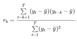
An Auto Correlation Function (ACF) Plot (or Autocorrelation plot or correlogram) correlation plot of a time series. The ACF is a good graph to identify the order of an MA(q) process. A ‘cut off’ (meaning a steep drop) indicates the best q in a MA(q) model.
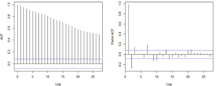
Interpreting the Auto Correlation Function (ACF) Graph
Here are a few points to keep in mind while reading an Auto Correlation Function (ACF) graph:
- A quick drop in the ACF is typical of a stationary time series (has no trend).
- A very slow, linear drop in the ACF pattern is typical of a nonstationary time series (has trend).
- An ACF plot that shows no pattern at all or up and down ACF plot is an indication of a series that shows no autocorrelation and is also referred to as “white noise.”
- Patterns such as waves in an ACF plot indicate seasons.
As useful as the ACF is in identifying the best q in a MA(q) model, the ACF is not as useful in identifying the best p in an AR(p) model. It is the partial autocorrelation function PACF of the time series that is helpful in identifying the p in an AR(p) model.
The Partial Correlation Function (PACF)
The PACF graph is a plot of the partial correlation coefficients between points in a time series (lags). A PACF graph shows only the “partial” correlation between two variables and not the complete correlation. The PACF graph only keeps the correlation between the two data points considered as it removes the correlation of the data points in between! For example, the PACF between yt and yt-4 shows the correlation between yt and yt-4 after removing the correlation between yt and yt-1, yt-2 and yt-3.
An AR(p) model by definition means that yt is affected by the previous observations 𝑌𝑡−1…………… 𝑌𝑡−𝑝. Therefore, the ACF of 𝑌𝑡 and 𝑌(𝑡−𝑘) must automatically contain effects of 𝑌(𝑡−1),…,𝑌(𝑡−𝑘+1), the observations “in between”. The Partial Autocorrelation Function (PACF) of an AR(p) process at lag 𝑘 is the autocorrelation between 𝑌𝑡 and 𝑌(𝑡−𝑘) after removing the effects of 𝑌(𝑡−1),…,𝑌(𝑡−𝑘+1). The idea of the PACF is to run two linear regressions for 𝑌𝑡 and 𝑌(𝑡−𝑘) on 𝑌(𝑡−1),…,𝑌_(𝑡−𝑘+1), and then compute their residuals.
Interpreting the Partial Auto Correlation Function (PACF) Graph
Here are a few points to keep in mind while reading a Partial Auto Correlation Function (PACF) graph:
- The PACF graph is used to find the p in the AR(p) model.
- The 𝑃𝐴𝐶𝐹(𝑘) of an AR(p) process has a cut-off at 𝑝.
- The 𝑃𝐴𝐶𝐹(𝑘) of an MA(p) process has no cut-off and instead decays exponentially (fades gradually) or has damped sine wave pattern.
You can read more about interpreting the ACF and PACF graphs here.
Forecasting Textbooks
- Hanke, John E. and Wichern, Dean (2014). Business Forecasting (9e). Essex: Pearson Education Limited.
- Montgomery, D. C., Jennings, C. L., & Kulahci, M. (2015). Introduction to time series analysis and forecasting. New Jersey: John Wiley & Sons.
- Hyndman, R.J., & Athanasopoulos, G. (2018) Forecasting: Principles and Practice, 2nd edition, OTexts: Melbourne, Australia
- A Very Short Course on Time Series Analysis by Roger Peng
Note” A white noise series is where we see 95% of the spikes in the ACF to lie within ±2/√T±2/T where T is the length of the time. Learn more about white noise here.
ARIMA Resources
- Open Text ARIMA Chapter from Forecasting: Principles and Practice
- Duke’s ARIMA pages
- Penn State’s ARIMA pages
- ARIMA Forecasting Using Python
- ARIMA Forecasting Using Python (2)
- ARIMA modeling in R
Enjoy learning! Do call or email if we can assist you with tutoring for Auto-Regressive Integrated Moving Average (ARIMA) Forecasting.