You can’t have missed hearing about how R and Python are two of the best languages to learn for a data science career.
According to the 2017 Burtch Works Survey, out of all surveyed data scientists, 40% prefer R, 34% prefer SAS and 26% Python. According to KDNuggets’ 18th annual poll of data science software usage, R is the second most popular language in data science.
What we have noticed in the last few years is that more business schools are incorporating R programming into their statistics and data analysis courses. Some only provide a cursory look at it but a few others have their entire statistics and data analysis courses implemented in R programming. We find that it is not just business schools but other departments including the humanities and engineering departments that have been teaching more data analysis using R programming.
We have been tutoring statistics, operations and data analysis courses at the graduate and undergraduate levels for over 10 years. Almost all courses were based on Microsoft Excel and had varying degrees of specialized software such as SPSS, SAS, @Risk, Crystal Ball, etc. Given the increasing prominence of data analysis using R programming in business schools, we have built resources to tutor students in data analysis using R programming. We will be happy to provide you live tutoring for your specific R programming project or class. Email or call us or simply fill out the sign-up form below to start live one-on-one statistics tutoring.
Some of the factors that contribute to the popularity of R are:
- It is free and open-source software.
- New libraries are constantly being developed by users. R and its associated libraries allow even beginners in data science to employ statistical techniques like linear regression, classification, resampling, linear model selection and graphical representation of data. As of now, the CRAN package repository holds 12098 available packages. These can be downloaded from here.
- R has an extensive library of tools for data wrangling. Data wrangling refers to cleaning up data sets so that they can be analysed.
- A lot of resources that are available for learning statistics/data science use R, rather than Python. As such, for a person with no coding experience, it might be better to start learning data science with R . However, resources like books and MOOCs that teach statistics/data science with Python do exist.
How do you get started with R? What is a typical learning path for a student of R?
- Download R and RStudio.
- Read “An Introduction to R” by W. N. Venables, D. M. Smith and the R-core team. It can be downloaded for free from the CRAN project website.
- Read “R for Data Science” by Hadley Wickham and Garrett Grolemund.
You will learn how to use R tools to do data visualization, data transformation and exploratory data analysis. “R for Data Science” is available free online at http://r4ds.had.co.nz/. - Some other free online courses and books are listed below:
Datacamp has a free R tutorial at https://www.datacamp.com/courses/free-introduction-to-r.
Code School has a free R tutorial at http://tryr.codeschool.com/.
http://www.cookbook-r.com/ is a compact book that gives you a quick review of R. - Data for an R student:
Once you have learned the basics of R, it is time to practice on datasets. Datasets can be downloaded from:
http://asdfree.com/ ( for survey data)
https://www.kaggle.com/
http://www.kdnuggets.com/datasets/index.html
https://data.worldbank.org/Example:
Let us work on the “Cycle Share” dataset which can be downloaded from :
https://www.kaggle.com/pronto/cycle-share-dataset
Source: https://www.kaggle.com/pronto/cycle-share-dataset
It consists of 3 files, “station.csv”, “trip.csv” and “weather.csv”.
The first step is to read in the data. Assume the “trip.csv” and “weather.csv” files are stored on your desktop.
The following lines read these files into R.
trip=read.csv(“……/Desktop/trip.csv”,stringsAsFactors=F, na.strings=””)
weather=read.csv(“……/Desktop/weather.csv”,stringsAsFactors=F, na.strings=””)
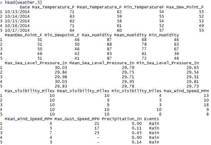
Now , to take a look at the first 5 rows of the objects “trip” and weather”, “head()” can be used as “head(trip, 5)” and “head(weather,5)”. This will give you an idea of the different columns in these two datasets.
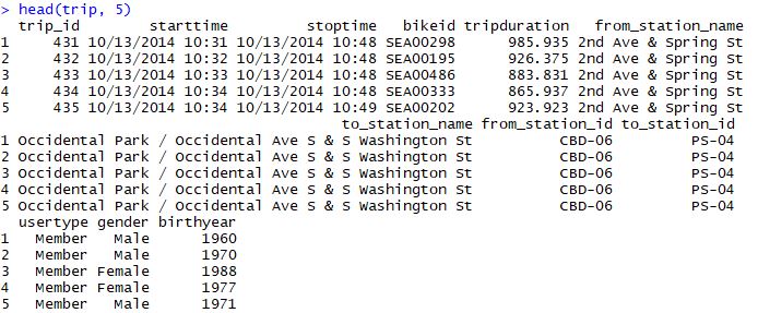
Please note that R is case-sensitive. So please remember not to write the code as “head(Trip, 5)” since you have already named the object “trip”.
> head(Trip, 5)
Error in head(Trip, 5) : object ‘Trip’ not found
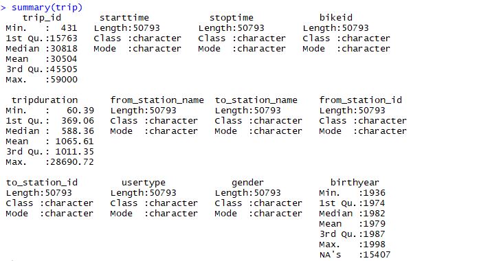
To get a summary of the different columns in “trip”, the “summary” function can be used.
We can also use the “summary” function to get a summary of the individual columns in “trip.csv”. For instance, the code “summary(trip$tripduration)” gives a summary of the “tripduration” column in the “trip” dataset.
> summary(trip$tripduration)
Min. 1st Qu. Median Mean 3rd Qu. Max.
60.39 369.10 588.40 1066.00 1011.00 28690.00
Let us classify the “tripduration” values as “long” ( if it is more than 1011.00), “medium” ( if it is more than 369.10 and less than or equal to 1011.00 ) and “short” (if it is less than 369.10 ).
trip$durationtype[trip$tripduration> 1011.00 ]=”long”
trip$durationtype[trip$tripduration>369.10 & trip$tripduration<=1011.00 ]=”medium”
trip$durationtype[trip$tripduration< 369.10 ]=”short”
A new column called “durationtype” has been created by running the above lines of code.
Now, take a look at the “durationtype” column using the “table” function.
> table(trip$durationtype)
long medium short
12705 25388 12700
This shows that 12705, 25388 and 12700 trips are classified as “long”, “medium” and “short”, respectively.
How can we combine the “trip” and “weather” datasets ? This could be done by merging the datasets if both of them had a “date” column. But the “trip” dataset has a “starttime” variable whereas the “weather” dataset has a “Date” variable. So these two variables have to be standardized.
> typeof(trip$starttime)
[1] “character”
> trip$time1 = strptime(trip$starttime, format = ‘%m/%d/%Y %H:%M’)
> typeof( trip$time1)
[1] “list”
The first line of the above code “typeof(trip$starttime)” shows that trip$starttime is of type “character”. The “strptime” command converts a string into a time data type. It also requires a format string given as “format = ‘%m/%d/%Y %H:%M’” as this is the format of the “starttime” variable. Thus, we get the “time1” variable.
Now, we would like to extract only the date from the “starttime” variable . For this , we can use the “strptime” command , but with the format string given as “format = ‘%m/%d/%Y’ ”.
> trip$date = strptime(trip$starttime, format = ‘%m/%d/%Y’)
Thus, we get the “date” variable with only the date.
Now, we look at the “Date” variable in the “weather” dataset.
> typeof( weather$Date)
[1] “character”
As it is a string, we use the “strptime” command , with the format string given as “format = ‘%m/%d/%Y’ ” to convert it into a time data type.
> weather$date = strptime(weather$Date, format = ‘%m/%d/%Y ‘)
Next, we use the “merge” command to merge the “trip” and “weather” datasets by the “date” column into a new dataset called “joint”.
> joint=merge(trip, weather,by=”date”,all=”TRUE”)
Looking at the “joint” dataset, we see that it has all the variables of the “trip” and “weather” datasets. Next, we extract the year, month and day from the “date” variable in the “joint” dataset using the “format” command.
> joint$year=format(joint$date,”%Y” )
> joint$month=format(joint$date,”%m” )
> joint$day=format(joint$date,”%d” )
Next, we would like to create a new column in the “joint” dataset called “age” which gives the age of the cyclist. This can be done by subtracting the “birthyear” variable from the “year” variable.
> joint$age=joint$year-joint$birthyear
Error in joint$year – joint$birthyear :
non-numeric argument to binary operator
However, the line of code “joint$age=joint$year-joint$birthyear” gives an error. Let us check why.
> is.numeric(joint$birthyear)
[1] TRUE
> is.numeric(joint$year)
[1] FALSE
We see that joint$year is not a numeric variable and must be converted into one using the “as.numeric” command before it can be used.
> joint$age=as.numeric(joint$year)-joint$birthyear
Now, the “summary(joint$age)” command gives the following result:
> summary(joint$age)
Min. 1st Qu. Median Mean 3rd Qu. Max. NA’s
16.00 28.00 32.00 35.35 41.00 78.00 15909
Next, we use the ggplot2 plotting system to visualize the data in the “joint” dataset.
> install.packages(“tidyverse”)
> library(tidyverse)
Now, we are going to prepare barplots of the data in the “joint” dataset with “durationtype”, “usertype”, “gender” and “gender” along the x-axis to get the plots below.
> ggplot(data = joint) + geom_bar(mapping = aes(x = durationtype))+ labs(y=”Count”, title = “Number of bike trips by durationtype”)
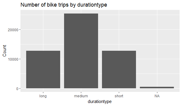
We see that most of the trips are of “medium” duration.
> ggplot(data = joint) + geom_bar(mapping = aes(x = usertype))+labs(y=”Count”, title = “Number of bike trips by usertype”)
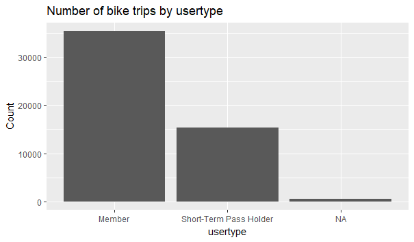
We see that “Members” take more than double the number of trips taken by “Short-Term Pass Holders”.
>ggplot(data = joint) + geom_bar(mapping = aes(x = gender))+labs( y=”Count”, title = “Number of bike trips by gender”)
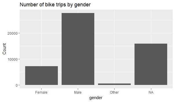
We see that most of the trips are taken by men.
>ggplot(data = joint) + geom_bar(mapping = aes(x = age))+labs( y=”Count”, title = “Number of bike trips by age”)
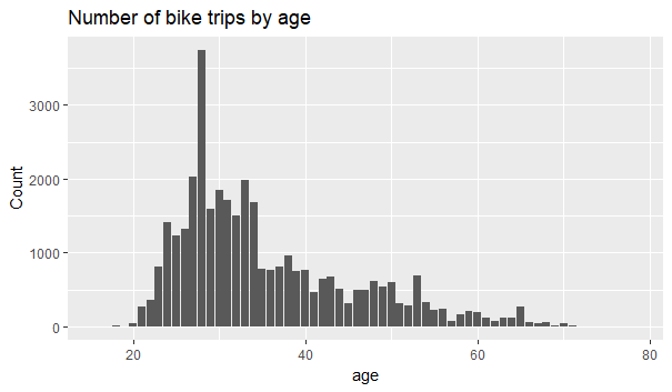
We see that most of the trips are taken by 28 year old individuals.
Thus, using the ggplot2 package and simple barplots, we are able to get a preliminary idea of the profile of the cyclists. Using this, we can decide how to proceed in order to learn more from this data.
This is an example of a specific task. We will be happy to provide you statistics tutoring for your specific R project or need. Email or call us or simply fill out the sign-up form below to start live one-on-one tutoring in data analysis using R.