In statistics, a measure of central tendency is a single value or number that attempts to describe or represent a data set by identifying the central position within that set of data. We can use a single value or number that attempts to describe or represent a set of data because most data tend to cluster around central points.

For example, it would be difficult to tell how a class performed by looking at a long list of hundred scores. On the other hand, by applying the measures of central tendency – the mean, median, or mode, we could get a typical or single number which would give us a better idea of the students’ performance. It would also help us compare this class with other classes. So instead of reading out 100 scores, we could simply say that the class average is 85%. The average is another term for the mean – a measure of central tendency.

Measures of central tendency are sometimes called measures of central location. They are also classified as summary statistics. Informally, measures of central tendency are sometimes also called averages. This page should help you to:

1. understand the concept of central tendency.
2. understand the purpose of the measures central tendency.
3. learn how to compute and use the measures of central tendency.
4. understand the advantages and disadvantages of the different measures of central tendency.

What are the Measures of Central Tendency?

The three most common measures of central tendency are the mean, median, and mode. Each of these measures calculates the location of the central point using a different method. The choice of a measure of central tendency depends on the type of data at hand.

Mean – The most popular measure of Central Tendency

Often called the average, the mean is the most familiar measure of central tendency.  It is the sum of all the data points divided by the number of data points.

The arithmetic mean is the central value of a set of numbers in a data set. It is used with both discrete and continuous data, although it is most often used with continuous data. The mean is equal to the sum of all the values in the data set divided by the number of values in the data set.

The formula to compute the mean:

                     the sum of the terms

   Mean =    ———————–

                    number of  terms

Sample mean and population Mean: A sample is just a small part of a whole. For example, if we need to know how much people pay for food in a year, we need not survey over 300 million people. Instead, we will take a fraction of that 300 million – maybe one thousand people. The fraction that is being considered is called a sample.

The mean is another word for “average.” So in this example, the sample mean would be the average amount those thousand people pay for food in a year. The sample mean is indicated by the symbol x̅ (pronounced X-bar). 

The formula to compute the sample mean:
x̄ = ( Σ x_i ) / n

The sample mean is useful because it allows us to estimate what the whole population is doing without surveying everyone. In statistics, samples and populations have different meanings.  These differences are very important, even if, as in the case of the mean, they are calculated in the same way.

To indicate that we are calculating the population mean, we use the Greek symbol “μ” (pronounced “mu”).

The formula to compute the population mean:

μ = ΣX/N

where ΣX is the sum of all the numbers in the population and N is the number of numbers in the population.

An important property of the mean is that it includes every value in a data set as part of the calculation. Additionally, the mean is the only measure of central tendency where the sum of the deviations of each value from the mean is always zero.

On the other hand, the one main disadvantage of the mean is its susceptibility to the influence of outliers.

Outliers:  Outliers are values that are unusual compared to the rest of the data set by being especially small or large in numerical value. For example, consider the wages of staff at a factory below:

Staff	1	2	3	4	5	6	7	8	9	10
Salary	15k	18k	16k	14k	15k	15k	12k	17k	90k	95k

The mean salary for these ten staff is Rs. 30,700. However, examining the raw data suggests that this mean value might not be the best way to reflect the typical salary accurately. While most workers in the data set have salaries in the Rs. 12k to 18k ranges, two of them have much higher salaries. Therefore the mean is being skewed by the two large salaries.

As the data becomes skewed, the mean loses its ability to provide the best central location for the data because the skewed data is dragging it away from the typical value.

Median

The Median is the middle number in a sorted list of numbers. It is the value that separates the higher half from the lower half of a data sample. In a data set, it may be thought of as the “middle” value. For example, in the data set [1, 2, 3, 6, 7, 8, 9], the median is 6, the fourth largest, and the fourth-smallest number.

Therefore, if the data set has an odd number of values, the median is the center value.  But, when there is an even number of values in a data set, the two middle values need to be added and divided by 2.  For example, in the data set [1, 2, 3, 5, 6, 7, 8, 9], the median is 5.5.

To determine the median value in a data set, the numbers must first be sorted or arranged in order of magnitude. As a result, the median is less affected by outliers and skewed data.  This property makes it a better option than the mean as a measure of central tendency.

The Mode 

The mode is the number that appears most frequently in a data set. A set of numbers may have one mode, more than one mode – bimodal, or no mode at all. 

 To find the mode, arrange the numbers in order of magnitude (from least to greatest), then count how many times each number occurs. The number that occurs the most is the mode.

For example, the data set below gives the retirement age of 11 people, in whole years:

54, 54, 54, 55, 56, 57, 57, 58, 58, 60, 60

Frequency table: This table shows a simple frequency distribution of the retirement age data. Such a table is known as the frequency table. The frequency table is created by arranging collected data values and their corresponding frequencies. The purpose of constructing this table is to show the number of times a value occurs.

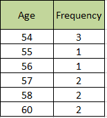
The most commonly occurring value is 54; therefore, the mode of this distribution is 54 years. 

Histogram: The graphical representation of a frequency table is called a histogram. On a histogram or bar chart, the mode is represented by the highest bar.

The mode has an advantage over the median and the mean. The mode can be calculated for both numerical and categorical (non-numerical) data. 

However, the mode has its limitations too. In some distributions, the mode may not reflect the center of the distribution very well. For example, when the distribution of retirement age is ordered from lowest to the highest value, it is easy to see that the center of the distribution is 57 years, but the mode is lower, at 54 years. 

54, 54, 54, 55, 56, 57, 57, 58, 58, 60, 60

It is also possible that there could be more than one mode – bi-modal or multi-modal in a data set. The presence of more than one mode can limit the ability of the mode to describe the center or typical value of the distribution because a single value cannot be identified to describe the center.

In some cases, particularly where the data are continuous, the distribution may have no mode (i.e., if all values are different).  In such cases, it may be better to consider using the median or mean, or group the data into appropriate intervals, and find the modal class. 

Advantages and disadvantages of the different measures of central tendency:

The mean, median and mode are all valid measures of central tendency. However, some measures of central tendency become more appropriate to use than others under different conditions. Such as:

The mean is the only measure of central tendency where the sum of the deviations of each value from the mean is always zero. On the other hand, the one main disadvantage of the mean is its susceptibility to the influence of outliers. As the data becomes skewed, the mean loses its ability to provide the best central location because the skewed data is dragging it away from the typical value.

The median is less affected by outliers and skewed data.  This property makes it a better option than the mean as a measure of central tendency.

The mode has an advantage over the median and the mean because it can be computed for both numerical and categorical (non-numerical) data. However, the mode has its limitations too. In some distributions, the mode may not reflect the center of the distribution very well. The presence of more than one mode can limit the ability of the mode to describe the center or typical value of the distribution because a single value cannot be identified to describe the center. In some cases, particularly where the data are continuous, the distribution may have no mode (i.e., if all values are different).  In such cases, it may be better to consider using the median or mean, or group the data into appropriate intervals, and find the modal class.

Summary of the Measures of Central Tendency

Central tendency refers to the measure used to determine the “center” of a distribution of data. It is used to identify a single value that represents an entire data set the most. The major types of central tendency are the mean, median, and mode.

The mean is 

• A single value that is intended to represent an entire set of data.
• It attempts to identify a central position (middle) within a data set.
• The mean is sensitive to outliers or skewed data.

The Median is

• The middle value of a sorted set of numbers.
• To determine the median we need to first sort or arrange the values of a data set in order of magnitude.
• The median is computed differently in the case of odd and even numbers of values in a data set.
• The median is not sensitive to outliers or skewed data. It is a better measure of central tendency when there are extremely large or small values in a data set.

The Mode is

• The most frequently occurring value in a data set.
• In a data set, a value can occur more than once or many times.  In such a case the data set will have 2 or more modes. This data set is then described as bi-modal or multi-modal.