We love MBA students! The life of an MBA student isn’t easy – it is plenty of hard work. Executive MBA students have it especially hard given that they have to manage the MBA challenge in addition to juggling their full time jobs and family commitments. Our mission is to make the lives of MBA students easier by “Making Learning Easier” (it is our motto – remember!)
And helping MBA students get their job done faster is part of “Making Learning Easier“. If you can finish something you needed to do in 30 minutes instead of an hour, we have just created 30 more minutes that they can use to learn something, finish up pending work, help their spouse with some task, enjoy it with their family or simply get some much needed rest! And getting more proficient on Microsoft Excel will definitely enable you to finish something you needed to do in 30 minutes instead of an hour. That’s why we have our pre MBA Microsoft Excel boot camp, why we have freely shared the Microsoft Excel functions directory, listed out 60 Microsoft Excel functions for MBAs and Microsoft Excel shortcuts list. If that is too much to digest, we have made your life a little easier by sharing the Top 10 Microsoft Excel Tips for MBA Students for you to learn today to save you many many hours during your MBA program and plenty more during the rest of your career.
Top 10 Microsoft Excel Tips for MBAs
Net Present Value (NPV)
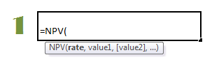 You will learn what the Net Present Value (“NPV”) concept means in detail in your first finance class and will likely use the concept in multiple classes throughout your MBA program (eg: DCF) and hopefully the rest of your life as you make investment or financial decisions. Net Present Value or NPV essentially shows you what a future stream of cash from is worth today given your ‘cost of capital’ or ‘discount rate’. We also have a lovely infographic that explains what the time value of money is. The Microsoft Excel syntax for the NPV function is “=NPV(discount rate, cashflow 1, cashflow 2, cashflow 3, ……)”.
Internal Rate Of Return (IRR)
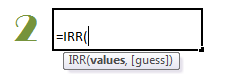 In your first finance class, you will also learn what the Internal Rate Of Return (“IRR”) means and along with the NPV use is often in multiple classes throughout your MBA program and hopefully the rest of your life as you make investment or financial decisions. The Internal Rate Of Return or IRR essentially tells you the effective interest you would have on a stream of payments. The Microsoft Excel syntax for the IRR function is = IRR(cashflow 1, cashflow 2, cashflow 3 … , discount rate guesstimate). In excel you will see it as “=IRR(values,guess)”.
‘PMT’ to Compute Loan Payments
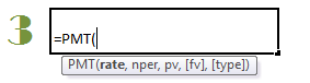 The Microsoft Excel ‘PMT’ function (which stands for ‘payment’) calculates the monthly or periodic payment for a loan or borrowing. This function is very useful to calculate the monthly payment on a home mortgage or a car loan. The Microsoft Excel ‘PMT’ function assumes that the payment will be a constant stream of payments at fixed period intervals of time and loan or borrowing with be at a constant rate of interest. The Microsoft Excel syntax for the PMT function is PMT(interest rate, number of periods, present value of the loan, future value of the loan, payment type-beginning or ending). In excel you will see it as “=PMT(rate,nper,pv,fv,type)”.
Pivot Tables & Charts
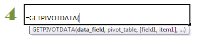 The pivot tables and charts feature in Microsoft Excel is arguably the single most useful tool. It quickly helps you summarize and analyze a larger or small set of data. This isn’t said lightly. By quickly, we mean in a matter of seconds! By summarize and analyze we mean almost any sort of statistical summary such as the count, sum, mean, etc. and what is fantastic is that you could categorize them in so many ways! Spending an hour learning this would save you at least a 100 hours over the course of your MBA program and possible 1000s of hours in your career if you were to work with excel. What is even better is that you can use specific outputs from Pivot tables as inputs in other parts of your excel spreadsheet or financial model. The Microsoft Excel syntax for the pivot table function is GETPIVOTDATA(data_field, pivot_table, [field1, item1, field2, item2], …) If this formula is complicated you can ignore this and simply enter =GETPIVOTDATA and link it to the cell in the PivotTable report whose content you want to pull out.
If function
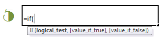 The If function is among the most versatile function of Microsoft Excel allowing you to model logical thinking into Microsoft Excel. The Microsoft Excel IF function first checks if the specified condition is true and if it is true specifies the outcome of the situation. If the function is not true or it is false, then the if function false, specifies another outcome for the situation. There is probably no limit to the uses and application of the IF function. You could have a single logic instruction alone or have multiple sets of logical functions built into one Microsoft Excel cell using the IF function (nested If functions). The IF function can be used alone or in combination with other Microsoft Excel functions. The Microsoft Excel syntax for the If function is IF(provide the logic you want to evaluate, [provide the outcome if the logic is true or satisfied], [provide the outcome if the logic is false or NOT satisfied]). Inside the Microsoft Excel cell you will see it as “= IF(logical_test, [value_if_true], [value_if_false])”.
VLOOKUP & HLOOKUP Functions
 The lookup functions VLOOKUP and HLOOKUP are also very handy. VLOOKUP stands for vertical look up where you ask Microsoft Excel to look up a value in a row (top to bottom) and pull out a corresponding cell’s contents from an array. HLOOKUP stands for horizontal look up where you ask Microsoft Excel to look up a value in a column (left to right) and pull out a corresponding cell’s contents from an array. The VLOOKUP and HLOOKUP are not to be confused with the lookup function which is also used for a similar purpose. We prefer the VLOOKUP and HLOOKUP as they are more robust and less error prone! The Microsoft Excel syntax for the VLOOKUP function is VLOOKUP (lookup the value, in this table array, and pull out the column number, specify if you want an exact match or if an approximate match is sufficient). Inside the Microsoft Excel cell you will see it as VLOOKUP(lookup_value, table_array, col_index_num, [range_lookup]). The Microsoft Excel syntax for the HLOOKUP function is HLOOKUP (lookup the value, in this table array, and pull out the column number, specify if you want an exact match or if an approximate match is sufficient). Inside the Microsoft Excel cell you will see it as HLOOKUP(lookup_value, table_array, col_index_num, [range_lookup]).
Fixed Reference / Absolute Reference
 The fixed reference also called absolute reference is a Microsoft Excel technique that you could definitely use on a daily basis! Fixed reference or absolute reference refers to the practice of linking to a ‘fixed’ or unchangeable cell when you are copying and moving formulas in a Microsoft Excel file. We use the fixed or absolute reference in a Microsoft Excel formula to refer to cells that we don’t want to change as the formula is copied and pasted elsewhere. The opposite of a fixed reference or absolute reference is called relative reference. When you provide a relative reference inside a formula, and we copy the contents of the formula and paste it elsewhere, it will not pick up the inputs from the original cell but from the same relative position in reference to the cell it is copied. When you use a formula that references the content in another cell the references are relative by default. To make it a fixed reference or absolute reference, so you would have to type dollar signs before the column alphabet and row number.
COUNT Functions
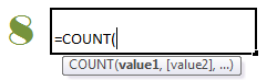 The COUNT family of functions is one that will be mightily useful for MBA students. The count function in Microsoft Excel includes the simple count function COUNT (specified range) counts the number of cells that contain numbers within the specified range. Inside the Microsoft Excel cell you will see it as “=COUNT(A1:A20)”. Other members of the COUNT family include COUNTA which counts the number of cells that are not empty inside a specified range of cells, COUNTBLANK which counts empty cells inside a specified range of cells, COUNTIF which counts the number of cells within a range that meet the given criteria.
SUM Functions
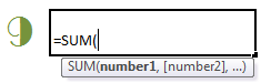 Just like the COUNT family of functions, the SUM family of functions will be mightily useful for MBA students. The sum function in Microsoft Excel includes the simple sum function SUM (specified range) sums up the values of cells that contain numbers within the specified range. Inside the Microsoft Excel cell you will see it as “=SUM(number1,[number2],…])”. Other members of the SUM family include SUMIF and SUMIFS which adds conditions to be satisfied before the values of cells that contain numbers within the specified range are added up. This family of functions is very useful for financial modeling and other types of operations modeling.
TREND function
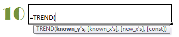 Making a judgment or decision on the future is an essential part of management. We need to forecast revenues, costs, capacity utilization, etc. using historical information. Most MBA students will encounter the regression technique and will spend time understanding the least square method of regression. Microsoft Excel has a nifty function called TREND. The TREND function generates the desired values for the decision assuming the trend (linear) continues along the established path. The Microsoft Excel TREND function fits a straight line using the same method used in a full blown regression analysis which is the least squared method. The Microsoft Excel TREND function is written with these instructions get the TREND(using the historical pattern of known_y’s and known_x’s and given me the corresponding values for a new set of day which is specified in a array new_x’s. Inside the Microsoft Excel cell you will see it as “=TREND(known_y’s,known_x’s,new_x’s,const)”.
Next Steps to Move Your Microsoft Excel Skills UP!
Those are our top 10 Microsoft Excel tips for MBA students. Of course, there are many more Microsoft Excel functions that are incredibly useful. You can find all the useful Microsoft Excel functions in our Microsoft Excel functions directory. If you want to prioritize learning these functions we have listed out the top 60 Microsoft Excel functions for MBAs too here. And PLEASE save yourself many hours by learning the Microsoft Excel shortcuts listed here. As always, remember the fastest way to learn Microsoft Excel. If we can help, please feel free to fill out the sign up form below or on the right sidebar.